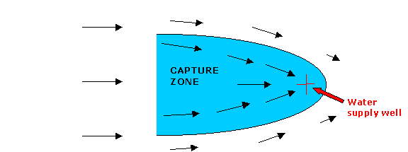
It is important to know where a domestic supply well draws groundwater
from, since this so-called capture zone may need to nbe protected to avoid
contamination of drinking water. One way to approach this problem
is to track the paths of hypothetical particles released from locations
upstream of the well as they are carried by groundwater moving towards
(or past) the well. This sketch shows typical groundwater velocity
vectors in the vicinity of a pumping well. A portion of the corresponding
capture zone is shaded.
Suppose that the velocity field is given (e.g. it may have been estimated
from water level measurements or simulated with a groundwater flow model).
We wish to write a MATLAB program to keep follow a number of particles
as they move from left to right.
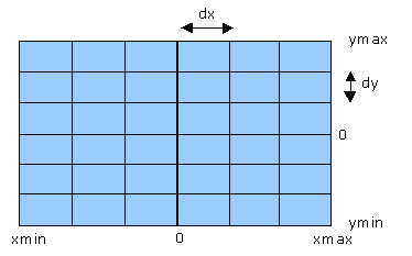
In this problem we need to consider variability over space as well as
time. This requires the definition of a rectangular
spatial grid
such as the one shown here. Velocities are defined at the intersections
of the grid lines (or nodes). The well is located at the origin
(x = 0, y = 0). Particles are released at specified (x,
y) coordinates at the initial time (t = 0). As the particles
move through the velocity field their x and y coordinates
change. These coordinates need to be recomputed at each time step.
The particles can be visualized by plotting their coordinates
as discrete points on an (x,y) graph which spans the computational grid.
Particles that leave the grid, either across the sides or through the well,
must be removed. Our objective is to plot the particles in a series
of snapshots taken at different times so we can see how they move towards
or past the well.
. 
The problem inputs are the number of grid points and the grid cell size,
the number of particles, the initial coordinates of each particle, the
time step, and the x and y components of the velocity at each grid node.
The velocities (which are computed within the program) depend on the well
location, the well pumping rate, the flow depth, and a specified regional
groundwater velocity. Outputs are the velocity components (which may be
plotted as vectors with the MATLAB quiver function) and particle
coordinates at specified times, which are plotted as an (x, y) scatter
plot (using the MATLAB
plot function).
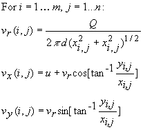
Two types of calculations are required for this problem: 1) calculation
of the velocity at each grid node and 2) calculation of the x and
y
coordinates of each particle at each time. The velocity at each node
is the sum of two components: 1) a regional velocity u, which we
assume is a constant pointing in the x direction and 2) the well
pumping velocity, which points radially towards the well. The well
pumping velocity component may be derived by applying the principle of
mass conservation. Suppose that the grid is viewed as an array, with
i
the row (or grid line aligned with the x direction) and
j
the column (or grid line aligned in the y direction). The
resulting equations for the
x and y velocities at node
(i,j) are:
where xi,j and yi,j are the x
and y coordinates of node (i,j).
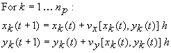
Once the x and y velocities are computed, the coordinates
of each particle at the new time (t+1) are related to the coordinates
at the old time (t) as follows:
where np is the number of particles and h is the
time step. The velocities at the old particle coordinates xk(t)
and yk(t) are obtained from the MATLAB grid interpolation
function interp2.
Translate the solution into MATLAB code: The downloadable
MATLAB code tracking.m solves the stated problem:
function tracking
% Program to simulate particle movement in
the capture zone of a
% pumping well
% Define velocity grid
nx=15
ny=15
u=1.5 % regional groundwater velocity
(constant in x direction)
Q=-20. % well pumping rate
dx=1. % x grid spacing
dy=1. % y grid spacing
d=1.
% flow depth
% define grid-related arrays
x=dx*[-(nx-1)/2:(nx-1)/2];
y=dy*[(ny-1)/2:-1:-(ny-1)/2];
xmin=x(1);
xmax=x(nx);
ymax=y(1);
ymin=y(ny);
% bigx and bigy define x and y corrdinates
respectively, of every % node in grid
bigx=ones(ny,1)*x;
bigy=y'*ones(1,nx);
% compute velocities (from mass balance)
denom=2*pi*d*sqrt(bigx.^2+bigy.^2); % radial
velocity denom.
zeroflag=(denom==0); %
check for divide by zero
denom(zeroflag)=1.; %
set zero elements of denom =1.
vr=Q./denom; %
compute vr
vr(zeroflag)=0.; %
reset vr = 0 where denom was originally zero
vx=u*ones(ny,nx)+vr.*cos(atan2(bigy,bigx));
vy=vr.*sin(atan2(bigy,bigx));
% plot velocity field
close all
figure
quiver(bigx,bigy,vx,vy)
axis([xmin, xmax, ymin, ymax])
% specify number of paricles and initial
locations
% y locations distributed randomly
np=100
yminp=ymin+0.10*(ymax-ymin);
ymaxp=ymin+0.90*(ymax-ymin);
xp(1:np)=x(2);
yp(1:np)=yminp*ones(1,np)+(ymaxp-yminp)*rand(1,np);
% specify number and size of tracking time
steps
nt=40
dt=0.5
% start time loop
for t=1:nt
k=1;
while (k<=np)
% interpolate velocities from
grid to particle locations
vxint=interp2(bigx,bigy,vx,xp(k),yp(k));
vyint=interp2(bigx,bigy,vy,xp(k),yp(k));
% compute
nominal new locations
ytemp=yp(k)+vyint*dt;
xtemp=xp(k)+vxint*dt;
% move particles
while they remain within grid
if(((xtemp~=0.)|(ytemp~=0.))&(xtemp>=xmin)&(xtemp<=xmax)...
&(ytemp>=ymin)&(ytemp<=ymax))
xp(k)=xtemp;
yp(k)=ytemp;
% remove particles
that have left domain
else
xp(k)=[];
yp(k)=[];
np=np-1
end
k=k+1;
end
% plot particle locations at
selected times
if((t==1)|(mod(t,2)==0))
figure
plot(xp,yp,'o')
axis([xmin, xmax, ymin, ymax])
else
end
end
return |
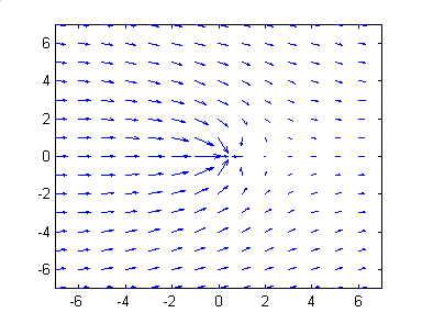
This program (with its internally specified inputs) produces the following
velocity plot.
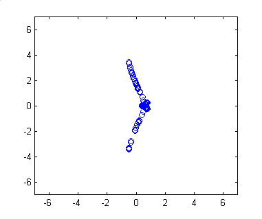
Here is a typical intermediate-time particle location plot for particles
originating from a line of vertical particles released on the left side
of the domain :
The easiest way to test this program is to modify the program inputs so
that we get a velocity field that moves the particles in obvious ways that
easily verified. For example, we should see all particles moving
horizontally in the limt as the well pumping rates goes to zero.in ways
thatou can do this yourself by replacing the inflows specified in the file
inflow.dat with other values. |