1. Conceptual model of diffusion (1 animation)
|
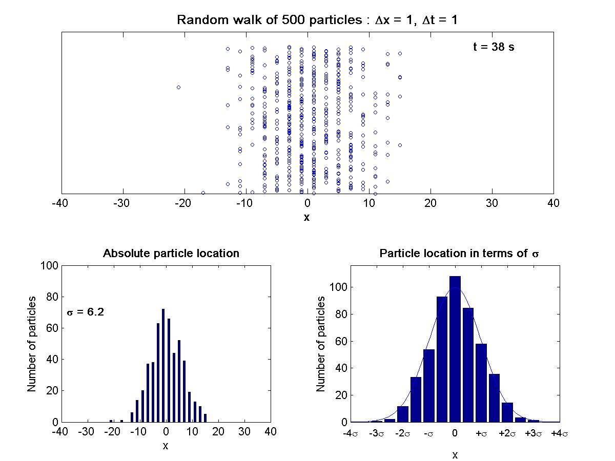
(a) RANDOM WALK ANIMATION
(click on image to begin animation) * If you are having trouble viewing this file, try saving it to your computer and opening it from there * Note to Unix users: the animation opens up behind active windows |
This animation shows the motion of 500 particles in a one-dimensional random walk with step size X = 1 in time t = 1. This random walk animation mimics the effect of Fickian Diffusion. For some background and thought problems pertaining to this animation, review the theory (page 4) behind this conceptual model of diffusion. |
Close window and return to mainpage
2. Conservation of mass (3 animations)
|
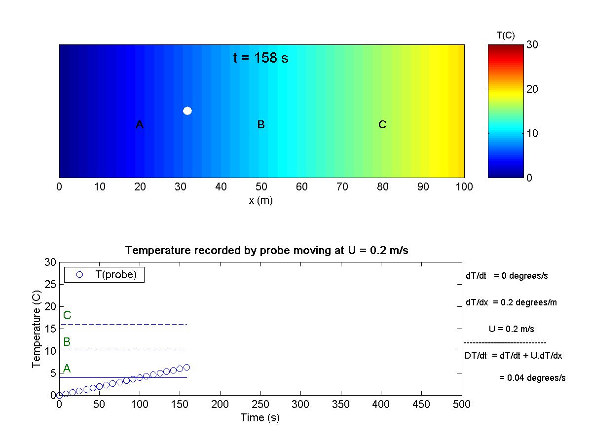
(a) ILLUSTRATION OF TOTAL DERIVATIVE: STEADY TEMPERA TURE FIELD
(click on image to begin animation) * If you are having trouble viewing this file, try saving it to your computer and opening it from there * Note to Unix users: the animation opens up behind active windows |
This animation shows a one-dimensional system with a spatial gradient of temperature, T(x). A temperature probe (white dot) moves with the flow, making a Lagrangian observation. The probe records the material (total) derivative. Go to the theory section (page 6) for some background material on the concept of the total derivative. |
|
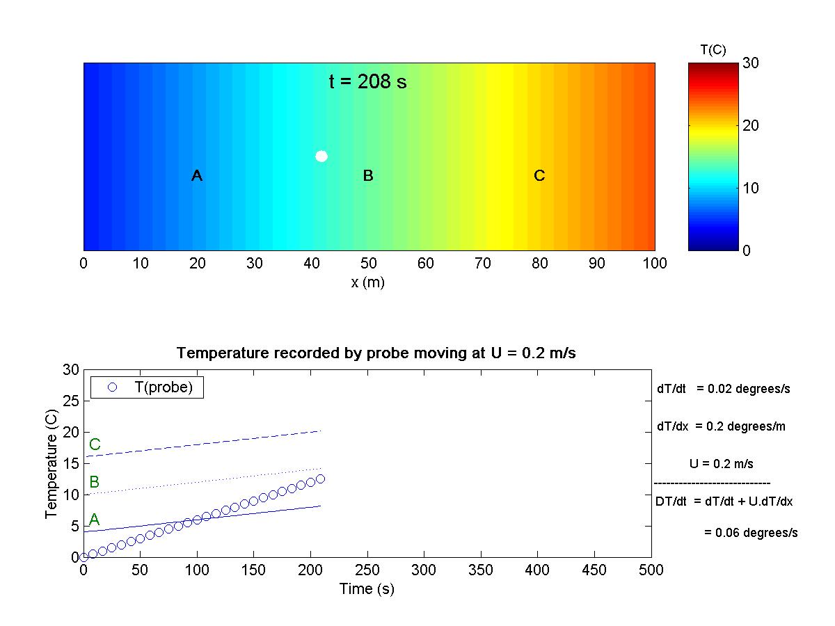
(b) ILLUSTRATION OF TOTAL DERIVATIVE: UNSTEADY TEMPERATURE FIELD
(click on image to begin animation) * If you are having trouble viewing this file, try saving it to your computer and opening it from there * Note to Unix users: the animation opens up behind active windows |
This animation shows a one-dimensional system with an unsteady temperature field, T(x,t). A temperature probe is moving through the flow at velocity u, and it records the material derivative. Three additional probes are located at the fixed positions A, B, and C. Go to the theory section (page 6) for some background material on the concept of the total derivative. |
|
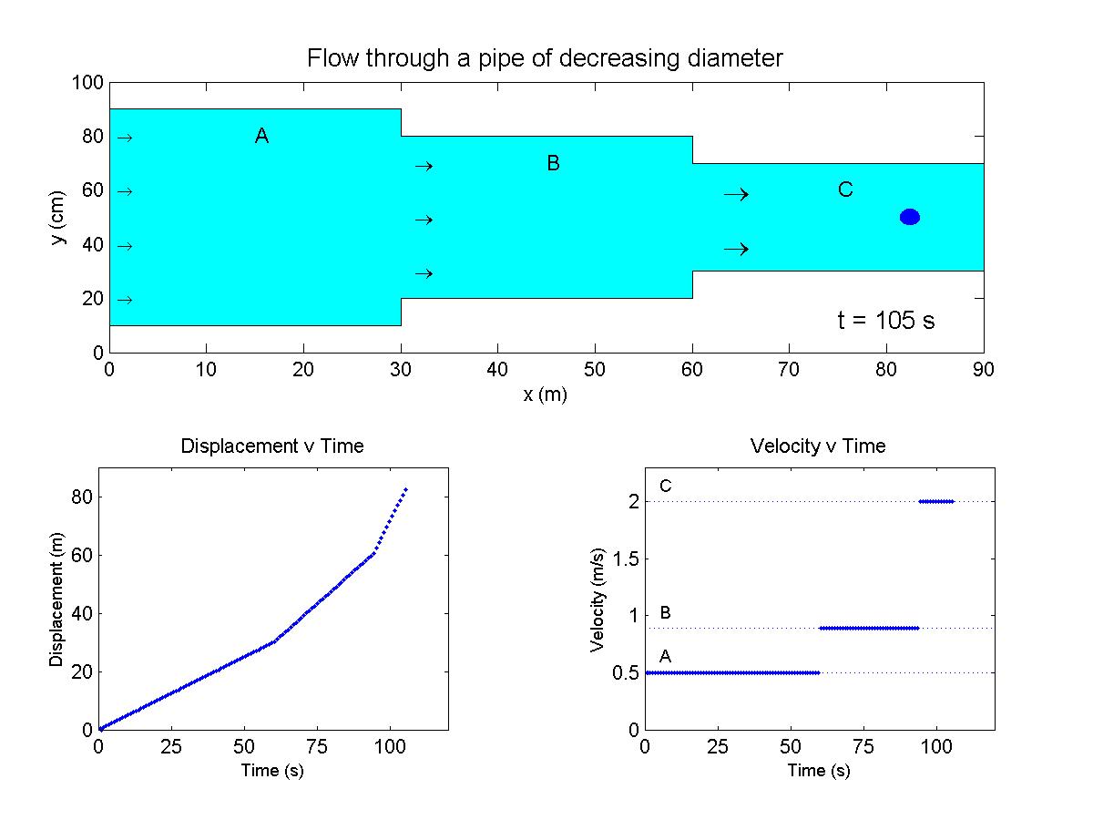
(c) STEADY, SPATIALLY ACCELERATING FLOW IN A PIPE
(click on image to begin animation) * If you are having trouble viewing this file, try saving it to your computer and opening it from there * Note to Unix users: the animation opens up behind active windows |
In this animation, flow through a pipe accelerates downstream as the pipe cross-section decreases. The velocity and displacement of a probe moving with the flow are shown versus time. For some background and thought problems pertaining to this animation, review the theory (page 6) behind spatially accelerating flows. |
Close window and return to mainpage
3. Diffusion of an instantaneous, point release (1 animation)
|
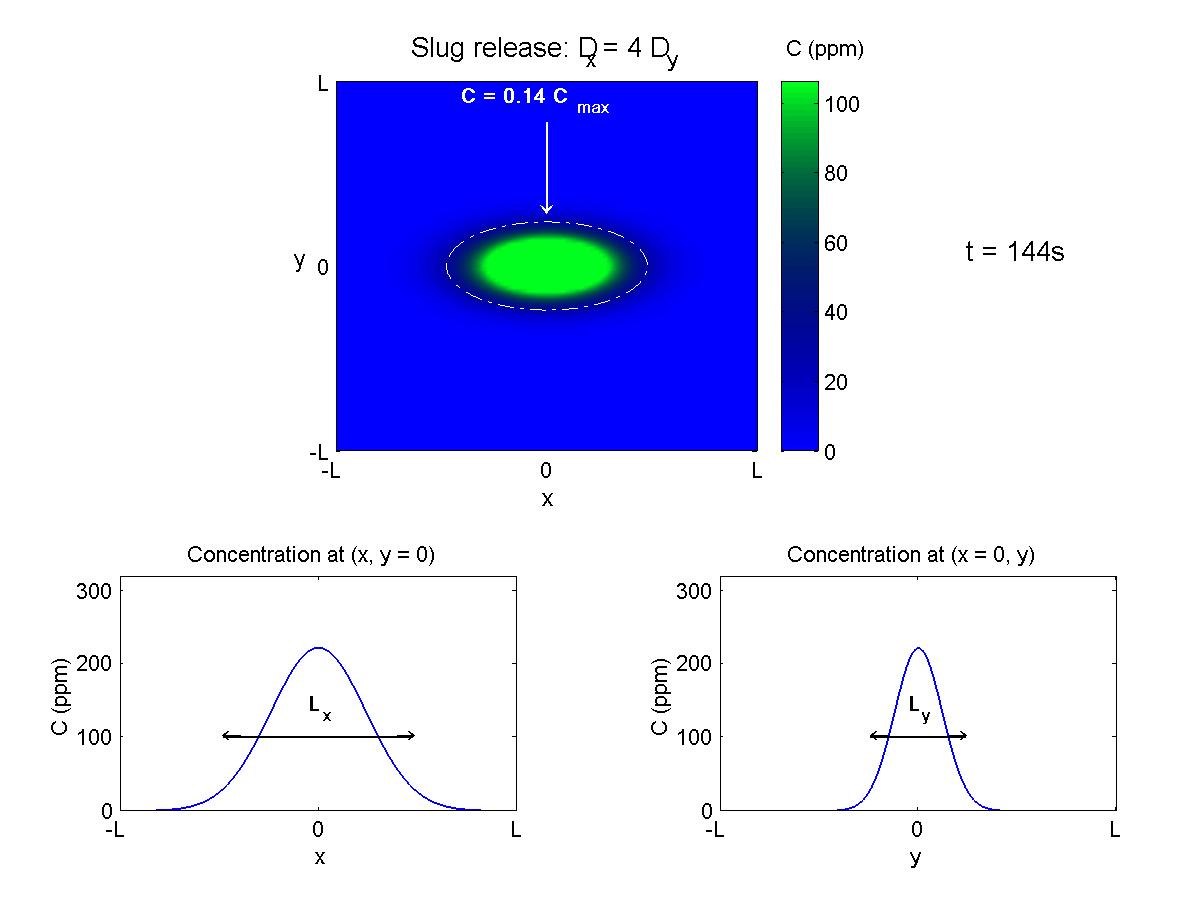
(a) ANISOTROPIC DIFFUSION IN TWO DIMENSIONS
(click on image to begin animation) * If you are having trouble viewing this file, try saving it to your computer and opening it from there * Note to Unix users: the animation opens up behind active windows |
This animation depicts the diffusion of a discrete mass released at (x = 0, y = 0, t = 0). The diffusion is anisotropic, Dx = 4 Dy. The length scales grow in proportion to the square root of the diffusion, such that the dimensions of the cloud are anisotropic, with Lx = 2 Ly. Note that the profiles of concentration along the x- and y-axes are Gaussian in shape. For some background and thought problems pertaining to this animation, review the theory (page 6) behind the diffusion of instantaneous, point releases. |
Close window and return to mainpage
4. Boundary conditions (1 animation)
|
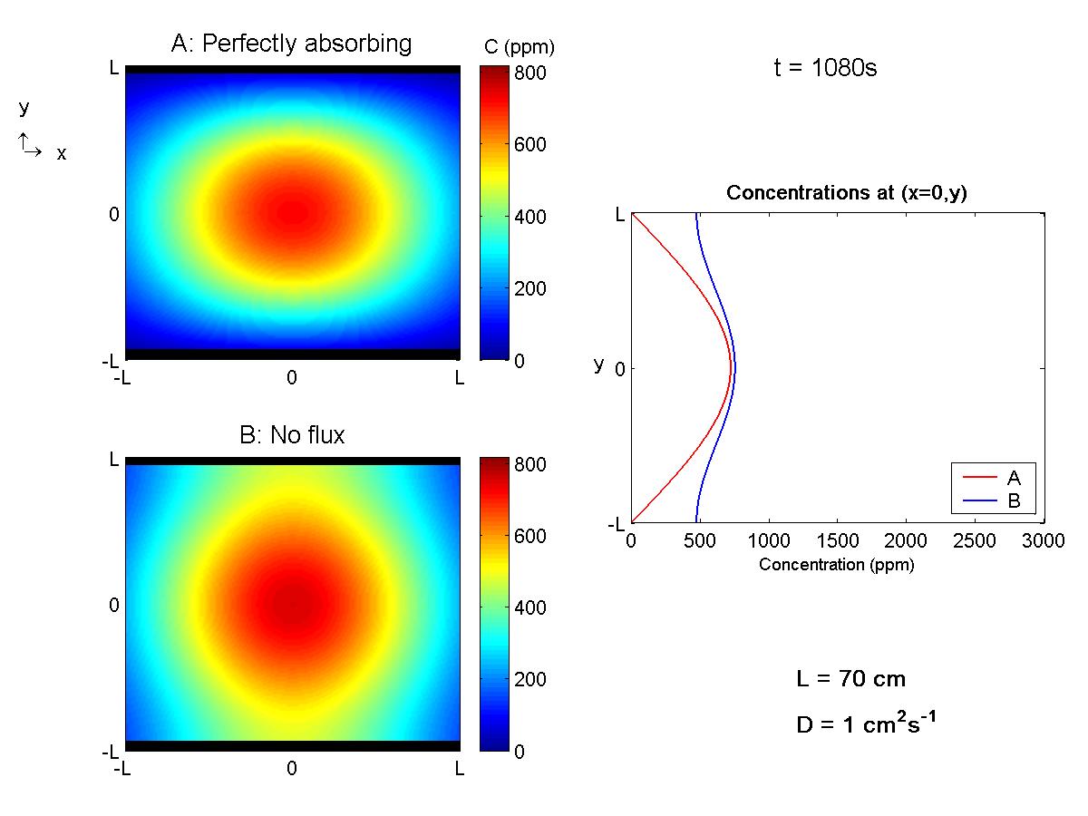
(a) COMPARISON OF NO-FLUX AND ABSORBING BOUNDARIES
(click on image to begin animation) * If you are having trouble viewing this file, try saving it to your computer and opening it from there * Note to Unix users: the animation opens up behind active windows |
The following animation examines the evolution of concentration after a slug mass is released mid-way between solid, parallel boundaries. Two scenarios are considered, perfectly absorbing and no-flux boundaries. For each system the concentration field is displayed in the plane z = 0. In addition, the concentration profile C(x = 0, y, z = 0) for each system is plotted for comparison on a single graph. For some background and thought problems pertaining to this animation, review the theory (page 8) behind modeling the effect of no-flux and perfectly absorbing boundaries. |
Close window and return to mainpage
5. Simultaneous advection and diffusion (1 animation)
|
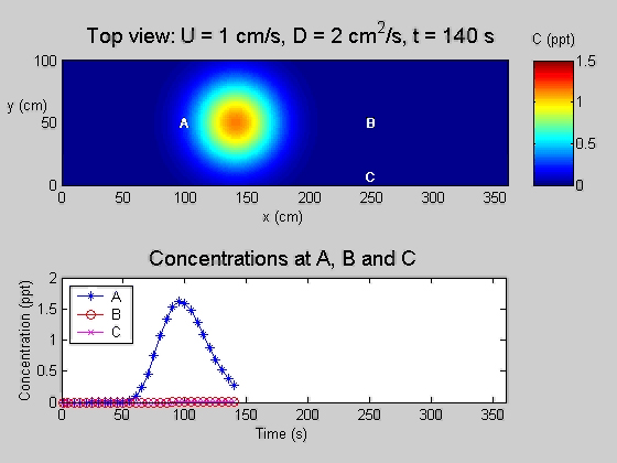
TEMPORAL RECORDS OF CONCENTRATION AS A DIFFUSING CLOUD PASSES BY
(click on image to begin animation) * If you are having trouble viewing this file, try saving it to your computer and opening it from there * Note to Unix users: the animation opens up behind active windows |
The following animation displays temporal records of concentration at three points after a mass is instantaneously released into a uniform flow. The concentration is Gaussian about the center of mass, which travels at a velocity U. The Peclet number of all measurement locations is high, so the maximum concentration is observed at roughly the advection time-scale. |
Close window and return to mainpage
6. Continuous sources(1 animation)
|
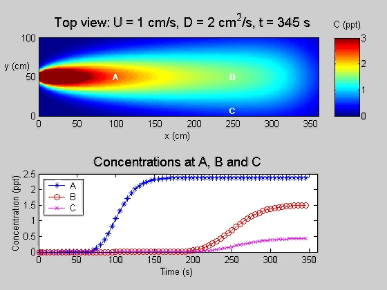
CONTINUOUS RELEASE INTO A UNIFORM FLOW
(click on image to begin animation) * If you are having trouble viewing this file, try saving it to your computer and opening it from there * Note to Unix users: the animation opens up behind active windows |
This animation depicts the evolution of the concentration
field downstream of a continuous point source in a channel with steady
flow (U = 1 cm/s). The concentration is measured at three points. At each
point the center of the front, defined by C = 0.5*Cfinal, arrives at the advection time scale, x/U. The duration of the front, which is the time required for the concentration to rise from C=0 to Cfinal, is 4 where |
Close window and return to mainpage