where the numbers zcomputed and ycomputed are close to the ztrue and ytrue that exactly solve your system of equations.
A*x = b
where A is a known mxn matrix, b is a known column vector with m entries, and x is the unknown column vector (with n entries). This is a compact way of writing down m linear equations in n unknowns. This is the most important type of equation in Chemical Engineering (and in most other engineering disciplines), so it is discussed in a lot of detail (and you will want to know most of the details).
In section 8.1 the necessary conditions on A and b for a solution to exist (and to be unique) are explained. In section 8.2 Gausss algorithm for solving this type of problem is detailed. Almost all important numerical methods are based on solving this problem, usually using variants of Gausss original algorithm, and solving Ax=b consumes a very large fraction of the worlds supercomputer cycles.
There are several ways one can run into technical problems. For example, the computed solution xcomputed may not be as accurate (i.e. not as close to the true solution xtrue) as you want it to be, and it may not be possible to do better. Sometimes the CPU time required to obtain a solution may be unacceptable, or (for problems with a large number of unknowns) the algorithm may require too much memory. All of these issues are discussed in section 8.3.
Modern matrix algorithms are oriented towards first factorizing the matrix into simpler forms, for example finding and lower triangular matrix L and an upper triangular matrix U such that L*U = A (L and U are called the factors of A). As discussed in Section 8.4, it is usually much easier to solve L*U*x = b numerically than it is to solve A*x=b.
Finally, in Section 8.5 a method for solving systems of nonlinear equations (including transcendental equations) by iteratively solving linear systems which approximate the nonlinear system is presented. (This is the famous algorithm developed by Sir Isaac Newton.) In 10.10 we will postpone discussing this until later in the semester.
We would then feed A and b as the inputs to our numerical equation solver,
and the solver would return as output a vector
where the numbers zcomputed and ycomputed are
close to the ztrue and ytrue that exactly solve your
system of equations.
Note that you could have written your equations in the opposite order without changing the answer. So you can freely permute the rows of A (as long as you simultaneously permute the numbers in b) without changing anything. You can also permute the columns of A (leaving b alone), and you will still get the correct numbers zcomputed and ycomputed back from the solver only this time the first number in xcomputed will be ycomputed, and the second one will be zcomputed. Do you see why?
For a more interesting and complicated example of going from a word problem to the correct standard form, see NMM Example 8.2.
For the important case where A is an NxN square matrix (number of equations = number of unknowns), and where all the columns of A are linearly independent (i.e. rank(A) is N), the columns of A span the full space RN, and you will get a consistent set of equations with any b. In this case you can be sure that the solution x will exist and be unique.
Ax=b is equivalent to:
x1A1 + x2A2 + x3A3 + ... + xNAN = b
where Ai means the ith column of A. This is also the same as
x1Am,1 + x2Am,2 + x3Am,3 + ... + xNAm,N = bm for m=1,2,3,...,N
Note that all the unknowns (the numbers xi) are on the left hand side.
Suppose A is upper triangular, i.e. all Am,j=0 if m>j. In particular, when m=N, only AN,N is non-zero. So for m=N there is only one nonzero term on the left hand side, and we can solve easily for xN:
xN = bN/AN,N
Now we know the numerical value of xN, the last term in the sum is known, so we can move the last term to the right hand side:
x1A1 + x2A2 + x3A3 + ... + xN-1AN-1 = b - xNAN= bN-1
well call the modified vector on the right hand side (still a list of numbers, no unknowns) bN-1, since we know its Nth entry is zero. Then we are back to almost the same situation as before:
x1Am,1 + x2Am,2 + x3Am,3 + ... + xN-1Am,N-1 = bN-1m for m=1,2,3,...,N-1
(m=N is not interesting anymore, since all of the terms on both sides are zero). We notice that for m=N-1, only the last term on the left hand side is nonzero. So we can solve easily for xN-1:
xN-1 = bN-1N-1/AN-1,N-1
Now we know the last term, so we can move it to the right hand side, and define
bN-1= b - xN-1AN-1
If we keep iterating in this way, we will gradually peel away at the terms on the left hand side until we know all the values in x.
A concise general algorithm implementing this procedure is given in
section 8.2.2, for either upper or lower triangular matrices.
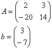
For example, if you had these two equations:
2z + 3y = 3
-20z +14y = -7
and you wanted to replace the second equation with an equation that did not involve z, you could multiply all the terms in the first equation by 10 and add the result:
20z + 30y = 30
to the second equation. Now your systems of equations is:
2z + 3y = 3
44y = 23
or in matrix form:

Now A is upper triangular!
Gauss proposed a systematic procedure for doing this so that the right unknowns will be eliminated from the right equations, so you can be sure that you will have a triangular matrix. The details are given in Section 8.2.3. This is important, you should read this carefully, and try it out by hand on a few small matrices to be sure you understand it.
Sometimes you have bad luck, and one of the numbers you need to divide by in these algorithms accidentally equals zero. More commonly, you will run into situations where you are called to divide by a very small number; this will not cause a disaster, but will exacerbate numerical round-off errors. To avoid this, methods with pivoting automatically permute the equations whenever necessary to avoid dividing by a small number. For details of how this is implemented, see 8.2.4. In practice, most people use the version called partial pivoting in the text.
In Matlab, to solve Ax=b, you just type
>> x=A\b
This simple command does the whole procedure (reduction to triangular form with partial pivoting, followed by solution of the triangular system of equations), see NMM 8.2.5
The equations in 8.3.2 show that a property of A, called the condition number, sets an upper bound on how much the errors in A and b could get amplified in computing x. In Matlab, cond(A) returns the condition number. If the condition number is large, we could be in big trouble. A horrendous case is shown in Example 8.9 where the condition number is 1014 and x is really not determined at all. More typically the condition numbers are maybe 103, and b might be known to 5 significant figures, with the result that xcomputed will be accurate to about 2 significant figures. (As a rule of thumb, for well-scaled x and b, see NMM 8.3.5, you lose about log10(cond(A)) significant figures in the arithmetic needed to compute x from A and b).
The key point is that A being poorly-conditioned (i.e. having a high condition number) is an intrinsic property of the system of equations we are using, it has nothing to do with the method we use to solve them (i.e. there is no way to get around it). If you get a super high condition number, it often means that you made a mistake in writing down the equations, e.g. you accidentally repeated an equation, or one of your equations is a linear combination of the others. If your equations come from experiments, and the condition number is large, it may indicate the experiment is poorly designed.
1*Mjar + 1000*mg_chemical = data1
1*Mjar + 0*mg_chemical = data2
you make the measurements, and find data1=9.0011 g and data2=9.0000
g
i.e.
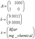
Note that x and b are both well-scaled (i.e. their entries have comparable magnitudes). Your boss wants to know the second component of x. You solve the system of equations by
>> x=A\b
and find x(2)=mg_chemical=11.000. Now you want to know how many significant figures you should tell your boss. You know that the numbers in A are perfectly accurate (since you believe mass is conserved, and there are exactly 1000 mg in a gram.) However, the numbers in b are only known to 5 significant figures (thats how good your balance is.) Now you can compute the approximate number of significant figures in x:
>> sigfigs = 5 - log10(cond(A))
or you could use the more detailed equations given in the textbook,
to get essentially the same result. What you find is that you can only
give your boss 2 significant figures, even though he gave you a 5-significant-figure
instrument. The poor experimental design in this example is using such
a heavy container: one would do much better by pouring the chemical into
a very light container with a weight comparable to or lighter than the
weight of the chemical. The way we are running the present experiment forces
us to subtract two larger numbers, a process which always kills off significant
figures.
If A*xcomputed?b, does that guarantee that xcomputed is close to xtrue?
The surprising answer, in NMM 8.3.4, is NO!. If cond(A) is large, all bets are off in that case there are many different xs which approximately solve the equation Ax=b. In some cases this is acceptable: you may not really care what x you use, as long as it approximately solves the equation. But sometimes, like the experimental example above, you really care what xtrue is; then poor conditioning is a disaster.
NMM 8.3.6 discusses how Matlab computes cond(A); if you are not curious
you should skip this section.
Ax = b
Aw = c
Av = d
and if A were a big matrix (say 1000x1000) we could save a lot of time by only computing U once, and by storing the operations that we are supposed to perform on the right hand side.
What Gaussian elimination is really doing is factoring A into two triangular matrices:
A = L*U where L is a lower triangular matrix. It is not hard to modify the algorithm so that you save L (as well as U). Once you have L and U, it is easy to solve the systems of equations:
Solve Ax=b by first solving
Ly=b for y
then solve
Ux=y for x.
For Aw=c, we just solve
Lq=c for q
And then solve
Uw = q for w.
At each stage you only need to solve a triangular system of equations, which is many times easier than solving a square system of equations. The details of the factorization procedure are given in NMM 8.4.; you dont need to know all the details, but you do need to get the general idea.
In reality, we will want to use partial pivoting to avoid dividing by zero or small numbers. So we will be permuting the rows of A and of b, and then finding the LU factors for the permuted A. In matrix language, we want to find P,L, and U given an A, where P is the correct permutation matrix (to avoid division by small numbers), and L and U are lower and upper triangular matrices:
P*A = L*U
Note that this L and U are different from what you would get without doing the row permutation, but they are the right ones for solving
P*A*x = P*b
Matlab provides a convenient LU factorization routine with partial pivoting:
>> [L,U,P] = lu(A)
You could use this to efficiently solve 2 similar systems of equations sequentially:
>> y = L\(P*b);
>> x = U\y;
>> q = L\(P*c);
>> w = U\q;
Matlab is smart enough to recognize that L and U are already triangular, so it will solve these equations very efficiently.
If you knew both b and c from the start, and you didnt plan to ever use L and U again, you could do this a different way: catenate b and c into a single matrix, and solve both problems simultaneously. In Matlab you would do it this way:
>> B = [b c];
>> X = A \ B;
>> x=X(:,1);
>> y=X(:,2);
Either way works fine, for about the same CPU time, but the first method has the advantage that you store L, U, and P for future use. Matlab is so smart that you actually do not need to save P (it will do the permutations automatically), for details see the discussion of lu.m towards the end of NMM 8.4.1, and the summary of what the backslash operator does in 8.4.3
NMM 8.5 covers Nonlinear Systems of Equations, which is really a very different topic; we will come back to this later in the semester.