Massachusetts Institute of Technology
Department of Urban Studies and Planning

Test Instructions

• This test starts at the 2:35 PM. You have until 4:55 PM to finish.
• This is an open-book, open-note test. However, do not contact any "live" non-staff person via electronic or other means while you take this test.
• There are 104 points total for the test. Question II-3C is a bonus question with an extra 4 points beyond 100.
• Please create your answers in electronic format - just as you have for lab assignments - and save your work, as usual, in your personal locker (i.e., the I:\ drive). You can edit your answers directly into your copy of this test if you have an HTML editor. For your convenience we have also provided MS-Word and PDF versions of the test in case you find these formats easier to work with.
• Even where we don't require an explanation, you may want to say a few words about what you did so that you can get partial credit if some of your numerical answers and names are incorrect but your method has merit.
• Turn in your test (both the text and the PDF exports of your maps) by uploading your answer documents to Stellar (just as you have done for homework). If you wish, you may open the answer sheet in MS-Word and include your PDF images within your answer sheet as a single document.
• Remember to turn in your test before leaving the room. Please confirm with an instructor that your exam has been received. We strongly recommend that you retain the file containing your answers until we return the graded exams to you.
• Make sure to include your name and Athena user ID near the beginning of each document that you turn in.
• Finally, don't spend all your time on one or two questions.Start by looking over all the questions to get a general sense of what, and how much, is being asked, and the grade points associated with each question--then start work on your answers. Move on to the next question if you've spent more than 10 minutes on any short answer question; mapping questions will likely take longer.

Good luck!

Datasets for the Test

For this test, we will use datasets, in the class data locker, from past homework and labs plus a new shapefile and one new data table in a personal geodatabase. All shapefiles represent locations using Massachusetts State Plane coordinates (NAD83) in meters. All the required datasets are in the class data locker in a folder called: S:\11.188\test19data (which is the same folder location as http://mit.edu/11.188/test19data). Here's a summary of the datasets you will use:

Filename	Description
ma_towns00type.shp	Shapefile from MassGIS of political boundaries for the 351 Massachusetts municipalities. This is the same as the ma_towns00 shapefule that we have used in past labs except that we have fixed the 'Gayhead' vs. 'Aquinnah' name problem and added additional attribute columns describing the community types to which the various Massachusetts municipalities have been assigned. The community type columns come from the table called MA_COMM_TYPE in the personal geodatabase (in MS-Access format) that is also provided to you. Since we have already joined the community type table to shapefile of Massachusetts municipalities, you will not need to use the ma_comm_type table in MS-Access. However, it could prove useful if you choose to answer some of the questions via MS-Access queries rather than ArcGIS data manipulation.
EXITS_PT.shp	Shapefile of points from MassGIS, that mark the location of all exits on limited-access highways (i.e., interstates and certain major State roads) in Massachusetts. Attributes include exit number and route number. you do not need additional information about the data layers but, if interested, further information is available from MassGIS at: http://www.mass.gov/anf/research-and-tech/it-serv-and-support/application-serv/office-of-geographic-information-massgis/datalayers/highwayexits.html.
11.188_test19gdb.mdb	A personal geodatabase (in MS-Access format) containing two tables (in addition to the GDB... tables that ArcGIS adds to MS-Access databases): MASS_DOR_COMPARE contains financial data about the 351 Massachusetts cities and towns that have been extracted from the 'Community Comparison Report' published annually by the MA Dept. of Revenue (DOR). These data are for Fiscal Year 2015 (fy2015) and include 25 fields describing town characteristics including property valuations and tax levys. A spreadsheet with the full set of fields available in the community comparison report is not needed for the test. However, for your information, the latest version of the report is here: https://dlsgateway.dor.state.ma.us/DLSReports/DLSReportViewer.aspx?ReportName=Comparative_Report MA_COMM_TYPE categorizes the 351 municipalities in Massachusetts into several 'Community Types.' The community types are distinguished by TYPE_CODE (with 9 categories) and a COMMUNITY_TYPE description (with 5 different labels). Other fields have the municipality names and codes in various numeric, text, upper case, etc. formats as well as the regional planning association associated with each municipality. The last two columns (MAPC and CTPS) indicate whether each municipality is a member of MAPC (in which case MAPC=1) and a member of CTPS (in which case CTPS=1). A data dictionary with further information about all the fields in each table is visible in MS-Access by viewing the 'design view' for the table. (Right-click on the table name in the table of contents and choose 'design view'.)
MASS_DOR_COMPARE.xlsx	A spreadsheet copy of the same MASS_DOR_COMPARE table saved in 11.188_test15_data.mdb. You can use either version to pull the table into ArcMap although it will be easier to do queries on the table if you work with the one in MS-Access.
11.188_test19_start.mxd	An ArcMap document to get you started with some of the shapefiles and tables that you will need for the test. Open it after copying the entire test19_data folder to C:\temp.

Before starting to use these datasets, you should copy the entire 'test19data' directory to a local drive (C:\temp in Room W31-301.) Using the data from your local drive will speed up the processing and ensure that you have write access to the files - just be sure to copy the whole directory back to your network locker (drive I) before you leave! Once you have copied the test19data directory to a local drive, run the ArcMap document, 11.188_test19_start.mxd that is in the directory. This ArcMap document will load the shapefiles that you need to get started.

Part I: Short Answers (46 Points)

Question I-1 (12 points total, 3 points each)

Using the MA_DOR_COMPARE table in MS-Access answer the following questions about Massachusetts municipalities::

• Which municipality has the highest equalized property value per capita (EQV12_PER_CAPITA) valuation? ___Chilmark____________
  What is that value? __3,624,181____________
• Which municipality has the lowest EQV12_PER_CAPITA valuation? ___Lawrence_________
  What is that value? _____39,482_________
• Which municipality has the highest density of road miles (road_miles13 / landarea)? ___Somerville_________
  What is that road density? ___25.82______
• Which municipality has the lowest density of road miles (road_miles13 / landarea)? ___Gosnold__________
  What is that road density? ____0.15____

Question I-2 (14 points total, 4+4+6 points)

Using the MA_COMM_TYPE table in MS-Access, or the same tabled joined into the Mass town map in the ma_towns00type shapefile, answer the following questions about the community type categorization of Massachusetts municipalities: (NOTE: There are 351 rows in the MA_COMM_TYPE table but 631 rows in ma_towns00type because (as we saw in Lab #4) municipalities with islands and rivers are split into more than one polygon.)

• How many of the 9 distinct 'type_code' values in MA_COMM_TYPE are associated with those Massachusetts municipalities that are in the Metropolitan Area Planning Council region (that is, MAPC=1)? __Of the 9 in total , 7 of them appear within the MAPC communities _____
• How many municipalities that are tagged with COMMUNITY_TYPE = 'Regional Urban Centers' fall within the 164 municipalities in Greater Boston that are affiliated with the Central Transportation Planning Staff (CTPS=1 in the MA_COMM_TYPE table)? ___In Access, construct a query from ma_comm_type that groups by type_code and community_type and counts the number of municipalities in each group but restricts the selection to those municipalities where CTPS=1. The number of municipalities in the CTPS region (containing a total of 164 municipalities) that are regional urban centers is: 21. If you do this computation in ArcMap, you must be careful to 'summarize' by municipality first since many towns have multiple polygons.

• Generate a table showing how many out of all 351 Massachusetts municipalities are in each community 'type_code' category? (Hint: If you do this in MS-Access, remember that you have to 'unhide' the 'Totals' option in the 'Query Design' tab in order to 'group by' a column in your output table.)

Community Types

TYPE_CODE	COMMUNITY_TYPE	CountOfCOMMUNITY_TYPE
1	Inner Core	7
2	Regional Urban Centers	34
3	Inner Core	9
4	Maturing Suburbs	22
5	Maturing Suburbs	41
6	Developing Suburbs	100
7	Developing Suburbs	55
8	Rural Towns	76
9	Regional Urban Centers	7

Question I-3 (20 points total, 5 points each)

Use the EXITS_PT shapefile in your ArcMap session and answer the following questions:

• How many municipalities contain at least one major highway exit? (Hint: Remember that one polygon/record in ma_towns00type does not necessarily equal one municipality so be sure to determine the number of unique municipalities that contain highway exits.) Number of municipalities = ___148______

Use 'select by location' to pick towns containing exits; open the attribute table if ma_towns00type and see that 151 rows are selected. However, there are 631 polygons in the layer since many towns are spread across several polygons due to rivers, islands, etc. You then need to 'summarize' the attribute table on the 'municipality' column and make sure to check the box that summarizes only for the selected set. Open this summarized table and see that there are 148 unique municipality rows.

• Next, we would like to count the number of major highway exits in each municipality. One way to get started with this calculation is to tag each row of the EXITS_PT attribute table with the name of the municipality that it falls within. Explain briefly the steps that you would take to do this using ArcGIS.

Do a spatial join of ma_towns00type into exits_pt to tag each exit with the name of the town containing it. Then summarize the attribute table for exits_pt on the town name or dor_code to get the number of exits that fall within each municipality.

• Carry out these steps in order to determine the number of highway exits within each municipality. Boston contains the largest number of exits (21) and Springfield is second with 15. Determine the municipality with the fourth largest number of major highway exits? town_name = ___Fall River____________
• What is the number of major highway exits that fall within that municipality? number of exits = ___13________

Part II: Spatial Analysis and Mapping Using ArcGIS (54 Points + 4 bonus points)

Question II-1 (38 points total)

Part II-1A (25 points): Develop a thematic map showing the equalized property value per capita (EQV12_PER_CAPITA) for each municipality. Turn in a PDF version of a properly annotated ArcMap layout of this thematic map using quantile classification with 10 categories.

• Display the major highway exits on top of the thematic map and show a 2 km buffer around the highway exits. (Beware: It may take a while to compute the buffer and even take up to a minute or so before any message window appears indicating the buffering is in process).
• Use a 50% transparency for the 2-km buffer so that the town boundaries and thematic shading are partly visible through the buffer areas. (Hint: A layer's transparency can be set with the transparency tool on the effects toolbar, or the 'Display' tab of a layer's 'Layer Properties' window.)
• Include on your map, a symbol for the location of each highway exits whereby the size of the symbol marking the location of the exit is graduated depending on the road density (road_miles13 / landarea) for the municipality in which the exit is located.
• Instead of showing all of Massachusetts, zoom in to Eastern Massachusetts so that your map focuses on the 164 towns in CTPS (that is, CTPS = 1 in ma_towns00type).
• Explain briefly your choice of color schemes, symbol size, and other cartographic choices in order to make the map more readable and appropriate to demonstrate any pattern that you discuss in the next question.

Point allocation <<< needs reconsideration...>>> Theme (4)
: EQV12_PER_CAPITA for each municipality; quantiles(10); range (39.5k-93.7k, ..., 671k-3.624k)
Layers (5): highway exits with 2 km buffer at 50% transparent
Symbology (5): exit symbol scaled to (road_miles13 / landarea) for its town; range: (2.2-5.0, ..., 14.0-25.8) quantiles(5)
Zoom (4): 164 Eastern Mass towns
Layout (4): with scale bar, source, north area, legend
Readbility (3) : annotated and nicely readable

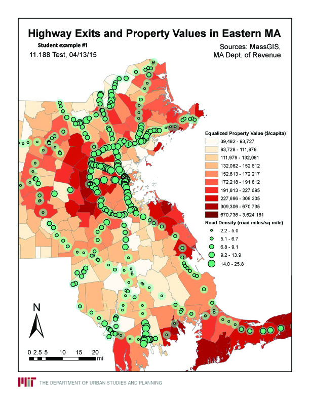
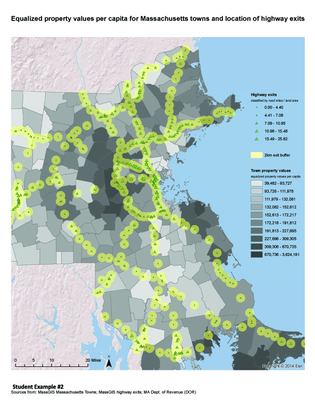
Map examples from student work: Both examples have the required features and annotations. The first example uses symbol sizes and color choices that make it especially readable, however, the range of values for road-density is incorrect. The second example has correct values but the symbol size for road density is scaled too large at the high end so the map is less readable in the vicinity of the exits. A few other adjustments for both maps would be desirable - but did not cost any point since we did not expect all of them given the time pressure of the test: (a) indicate data sources, (b) round off the legend values (as done in the second example) so irrelevant precision is not displayed, (c) indicate the classification method - e.g., 'Quantile classification', (d) indicate the units for road density (linear miles of road per aaa of land), and (e) correct for ArcMap symbol bias by displaying the squareroot of the road density using graduated symbols so the area of the symbol is proportional to the road density (instead of road density squared).

II-1a Map Example #1:

II-1a Map Example #2:

Part II-1B (8 points): Explain briefly what, if anything, your map seems to suggest regarding:

• The spatial pattern of road density and equalized property value per capita across Massachusetts?
• Any relationship between the location of highway exits and either road density or equalized property value per capita?

We see higher road density in the denser urban areas and lower road density in exurban aeas where equalized property value per capita are also low. The highest equalized property values are in close-in suburbs and (summer resort areas) - especially the western suburbs just beyond the first ring road (I-95, a.k.a. rt. 128) and, while some of those areas do not have a lot of exits, they are still within a few miles of the major interstates.

Part II-1C (5 points): Explain briefly a few pluses and minuses of using quantile classification to visualize the spatial distribution of equalized property value per capita among the 351 Massachusetts municipalities.

Quantile classification groups (approximately) the same number of features in each category. This approach helps the viewer differentiate the high/medium/low regions and is especially useful when percentile differences among spatial features are relevant. However, if the historgram of values is particularly skewed or lumpy, quantile classification can overemphasize differences between spatial regions (municipalities in our case) compared with 'natural' or equal interval grouping. When the actual value of the measure is more relevant than the ranking of municipalities, then one of the other classification schemes may be more appropriate.

Question II-2 (4 points total)

For this question, we would like to compare the relationship between per capita property values (EQV12_PER_CAPITA) and the percent of each municipality's budget that comes from state aid (STATE_PCT). Both values are availabble in MA_DOR_COMPARE. The median (50th percentile) value of EQV12_PER_CAPITA is $137677 and the median value of STATE_PCT is 10.79%.

Part II-2A (2 points): What are the average values of EQV12_PER_CAPITA and STATE_PCT for municipalities in which the STATE_PCT is greater than the median value (10.79%)? average of EQV12_PER_CAPITA = __$124963__ and average of STATE_PCT = ____23.09%____

Part II-2A (2 points): What are the average values of EQV12_PER_CAPITA and STATE_PCT for municipalities in which the STATE_PCT is less than the median value (10.79%)? average of EQV12_PER_CAPITA = __$279101____ and average of STATE_PCT = ____6.07%____

Question II-3 (4 points + 4 bonus points)

In ArcMap, select those municipalities that are in the Boston metro area (as indicated by CTPS=1 in MA_COMM_TYPE) and overlap any part of your 2 km buffer of the highway exits. (Hint: When you do a selection in ArcMap, you usually have a check box to specify whether to do a brand new selection or to select from the currently selected set.)

Part II-3A (2 points): How many polygons are in your selected set? The number of selected polygons = ____227 polygons within the 2 km buffer of exits and 144 polygons also in CTPS=1 municipalities_______________

Part II-3B (2 points): How many unique municipalities are in your selected set? (Remember from Lab exercise #4 that some municipalities have more than one polygon in the ma_towns00type.) The number of selected municipalities = _132 unique municipalities____________

Part II-3C (4 bonus points - beyond 100 points): Generate a scatterplot chart that plots EQV12_PER_CAPITA versus STATE_PCT for those selected municipalities (in the CTPS regions and overlapping the 2km buffer). (Be sure to show only one point per municipality.) Include a PDF of your chart in your test submission.

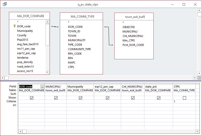
To generate this chart, start by using 'select by location' to select the 227 polygons in ma_towns00type that intersect the 2km buffer of highway exits. Then 'summarize' this table based on the 'MUNICIPALI' column to get one row per unique municipality. Before saving this summary table, click on the 'First' choice for the DOR_CODE field and 'Minimum' choice for the CTPS field. (Do you understand what these choices do?) In this way, you will add columns for CTPS and DOR_CODE in the output summary table. Those extra fields will be helpful in order to select towns within CTPS and to join the table to MA_DOR_COMPARE later on. If you save the summary table into the personal geodatabase 11.188_test19gdb.mdb, then you can open it using MS-Access and join to MA_DOR_COMPARE and MA_COMM_TYPE to select only the CTPS=1 towns and to get the eqv12_per_capita and state_pct values. Here is the query design:


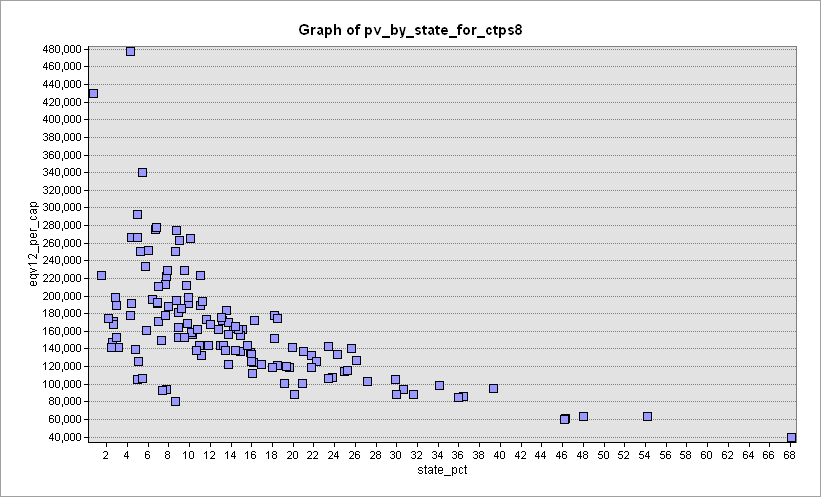
The result of this query is named 'pv_by_state_for_ctps8' and pulled into ArcMap from the personal geodatabase in order to draw the chart. Note the enormous various in property values per capita across the 132 towns in the chart. Those towns with high property values per capita tend to receive a small fraction of their town budget from state aid, whereas towns with low property values per capita tend to have the highest fraction of their budget consist of state aid. This is intentional since the State aid formulas try to give more money to towns who are least able to collect money through property taxes. The high-valued town at the top left is Weston, a wealthy Boston suburb with 400k per capita in valuation, and the low-valued town on the lower right is Lawrence, with just under $40k per capita.

Question II-4 (8 points): Coordinate Systems

Census tract boundary files that are available online from the US Census Bureau are typically expressed in a geographic coordinate system that encodes lattitude and longitude in decimal degrees. However, most state GIS agencies (such as MassGIS) provide census tract boundary files (and many other boundary files of interest to state agencies) in a projected coordinate system such as the NAD83 [meters], Massachusetts [Mainland] State Plane coordinate system that has been used for many of the shapefiles we have used in this class. Explain briefly at least two reasons why MassGIS users might prefer boundary files in Massachusetts State Plane coordinates and at least one reason why a national agency such as the US Census Bureau might prefer to distribute datasets in geographic coordinates (i.e., lat/lon).

First part: (1) Local agencies use projected coordinates with a projection method that keeps North straight up; (2) Local agencies use projections that do a better job of preserving distance measurements or areal measurements in the local area that is their focus of attention, and thereby avoid some of the distorations that arise when lat/lon values are plotted on a flat surface.

Second part: Latitude/Longitude measurement allows one consistent coordinate system to be used for measurements anywhere on Earth. However, plotting lat/lon as coordinates on a flat two-dimensional surface leads to distortions.

Please note:

• Before creating the PDFs, be sure to include your name and Athena ID somewhere on the map layouts
• Please test your PDF files with Adobe Acrobat Reader before submitting them to us in order to be sure they are readable.
• Keep a copy of your text output and PDFs file in your 11.188 user directory until your test is graded
• Confirm with an instructor that your test files were received?
• Turn in one text file (or Word or PDF document) with written answers to the questions, plus the map requested in Question II-1A and the chart in II-4C.

Back to the 11.188 Home Page.
Back to the CRN Home Page.