Note: We have swapped the labs labeled #4 and #5 (so this week is called #5)

You have two weeks to do today's lab (March 5) which is labeled Lab #5 on manipulating US Census data in MS-Access and ArcGIS. We will do Lab #4 (on data manipulation and charting in ArcGIS) next Monday and both labs will be due on Monday, March 16. This will give you a longer time to get comfortable with MS-Access and handling the large census tables. However, please to not put off both labs until next week! Also, keep in mind that homework set #1 is due this Wednesday (3.4) and the first part of homework set #2 will be due on Monday, March 16 (just before Spring Break).

Overview - Mapping the Percent of Workers in Metro Boston Who Drive to Work Alone

In this exercise you will use the American Community Survey (ACS) to create a thematic map indicating the percentage of workers in Eastern Mass block groups who drive alone to their jobs. The data about mode choice for workers comes from the 2009-2013 ACS data and the boundary files for Mass census block groups comes from the 2010 TIGERline files. Our final map will look similar to other thematic maps that we have generated, but it takes much more effort and understanding when the data sets are large and not already integrated with the map files. Planners are generally asking new questions that require finding and integrating new data in a manner appropriate for the question at hand. In this case, it takes some effort and understanding to identify and locate the relevant ACS variables, construct the appropriate indicator for each 2010 block group, and then join the new indicator to the block group map. This lab also covers new ground because you will be working with a different Census Bureau data product, the ACS, as opposed to the Decennial Census data that you've been working with up to this point. In 2000, the Census Bureau began phasing in the ACS to replace a large portion of the decennial Census. In 2010, the Census Bureau completed this task. The ACS is quite a bit different than the decennial census and it is well worth reading both the document we wrote and the first 12 pages of A Compass for Understanding and Using the American Community Survey: What General Data Users Need to Know.

In order to develop this map, you will have to create a table that contains the percentage of workers who drive alone to work (by car, truck, or van) for each block group in Boston Metropolitan Area. But the raw ACS data provide counts of the number of workers within each block group that use each transportation mode to get to work. Unlike the simple example (involving median earnings) shown in class, computing this percentage will require normalizing the ACS counts. (Here's a link to some additional discussion about when and how to >normalize> the data.).

The in-lab discussion notes are here: Lab #5 note.

Part I: Data and Resources for this Lab Exercise

Copy the zipped geodatabase to C:\temp

For this exercise, we will use a geodatabase that contains the geometry for 2010 Massachusetts Block Groups and and the 2009-2013 ACS data. You will also us one new shapefiles that provide boundaries for 2010 Massachusetts counties. The ACS uses census boundaries (e.g. block groups, tracts, etc.) of the most recent Decennial Census upon the data's release. Since we will be using 2009-2013 ACS data, we want to use 2010 block groups. The geodatabase is called: ACS_2013_5YR_BG_25.gdb (the file is compressed and will need to be "unzipped" before use) and the county shapefile is called: MA_County_2010.shp. The county file should be sourced as "2010 TIGER/Line Data." The geodatabasse should be sourced as "2010 Tiger/Line and 2009-2013 American Community Survey data." For your convenience, we have downloaded the county shapefile from the Census Bureau's TIGER/Line FTP site. We downloaded the geodatabase from a section in the Census Bureau's site that provides TIGER/Line data joined to selected demographic and economic data. For your convenience, we downloaded these files and placed them into the class locker, ./data/lab5_ACS_09_13/.We also included an ArcMap document, 11188_lab5_ACS.mxd, in that folder that loads the county shapfile, with relative path addresses, and includes several geospatial web services.

Before beginning the ArcMap work for this exercise, be sure to download the entire ./data/lab5_ACS_09_13 directory into C:\temp (or your flash drive or portable HD) and open your local copy of 11.188_lab5_ACS_09_13.mxd.

"Unzipping" the geodatabase and addding it to 11.188_lab5_ACS_09_13.mxd

Later in the Lab you will use the large (158 MB) geodatadatabase of 2009-2013 ACS, 5-year estimates and Massachusetts block groups. Before we can use this data, we need to "unzip" the file with the geodatabase. Using compression software (e.g. 7zip), "unzip" the file with the geodatabase, ACS_2013_5YR_BG_25.gdb, into a local directory. Next, open lab5_ACS.mxd, navigate to the location of the "unzipped" geodatabase, and add the geodatabase to the map.

Useful Resources:

• Notes and tutorials regarding the use of MS-Access
  • Last Wednesday's "Making Sense of the Census" lecture notes (and MS-Access demonstration) .
  • Additional notes and tutorials from that lecture and repeated here:
  • • START HERE if you are not familiar with MS-Access database management software
      • MS-Access 'recitation' notes by Lulu Xue and Shan Jiang: rec2_database_datafile.pdf
    • other useful online 'business skill' tutorials by The Goodwill Community Foundation of East North Carolina
      • The MS-Access tutorials are here: http://www.gcflearnfree.org/access2010
      • And, some useful pages on MS-Access query building are here:
        • http://www.gcflearnfree.org/access2010/8.2
    • MIT also subscribes to Skillsoft online training
      • How to us your (free) account:  https://ist.mit.edu/training/wbt
      • Skillsoft "Getting Started with Access 2007" course: http://www.skillsoft.com/catalog/detail.asp?CourseCode=mo_bgac_a01_dt_enus
      • Skillsoft provides training on many other topics including relational database design
• 2009-2013 ACS technical documentation
• Census Bureau geographic hierarchy/summary level charts
• Response rates for the ACS
• Information about geodatabases

---

Part II: Set the Coordinate System

If your ArcMap Data Frame is empty when you add the Massachusetts county shapefile, the Data Frame will display the data using Mass State Plane coordinates. However, depending upon which files you may already have loaded into your ArcMap session, the Block Groups layer may be displayed in geographic coordinates (lat/long) instead of the desired projection (using Mass State Plane coordinates). 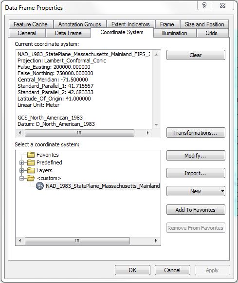If necessary, change the viewing projection in the Data Frame to "State Plane/NAD 1983/NAD_1983_StatePlane_Massachusetts_Mainland_FIPS_2001" from the "Coordinate System" tab in the Data Frame Property window. In “Select a coordinate system” window, expand “Projected Coordinate Systems”, followed by “State Plane”, “NAD 1993 (US Feet)”, and “NAD 1983 StatePlane Massachusetts Mainland FIPS 2001 (US Feet)”.

Add into ArcMap the MA_County_2010.shp shapefile of MA counties and the geometry for Massachusetts block groups ACS_2013_5YR_BG_25_MASSACHUSETTS located in ACS_2013_5YR_BG_25.gdb geodatabase. You can see what is in a geodatabase by navigating to the geodatabase in ArcMap (or ArcCatalog). Once you have navigated to the geodatabase, you can add a layer or table from the geodatabase to your map just like you would with a shapefile.

The block group geometry boundary file have no ACS data attributes - just the geographic identifiers that identify the block group. (Take a look by opening the attribute table.) Before we can compute the percentage of workers who drive alone to work, we need to find the relevant ACS data, add it into ArcMap, and join it (using the summary level-state-county-tract-block-group ID) to the block group data layer. Before doing this, we will focus on eastern Mass and export our own shapefile of the eastern MA block groups boundaries.

Let's change the names of our layers so that they are easier to use. Change the Massachusetts county layer to "Massachusetts Count Layer". Change the Massachusetts block group layer to "Massachusetts Block Group Layer".

Part III: Select Block Groups in the Boston Metropolitan Area and Export as your own Shapefile

STEP 1:

In order to work with a smaller file, we want to create a new shapefile that represents the Block Groups that fall within major Boston area counties (Essex, Middlesex, Worcester, Suffolk, Plymouth, Norfolk, Bristol, and Barnstable). We can select these block groups using the Select By Location tool in ArcMAP.

In the Massachusetts County layer, select Essex, Middlesex, Worcester, Suffolk, Plymouth, Norfolk, Bristol, and Branstable counties. If you are familiar with counties in Massachusetts, you can simply use the graphical selection tools to select the eight counties. If you aren't, use the Selection > Select By Attribute tool to select these eight counties by name from the attribute table of the county layer.

STEP 2:

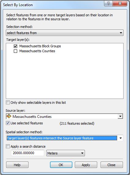
With the counties selected you are ready to use the Select By Location tool. This tool works on the currently active theme, so you will need to make sure the Massachusetts Block Groups Layer is active. Go to the Selection menu and select Select By Location.When the dialog window appears, choose to select features from your active layer (Massachusetts Block Groups 2010) using the spatial selection method "Target layer(s) features intersect with the Source layer feature" with the selected features of the Counties layer. Refer to the lab 3 for how to use the Select By Location tool. What problems might occur due to selecting features that intersect with the counties layer? Could you use "have their centroids within" selection option instead? What problems might that cause? Since Census blocks add up to Census block groups which add up to Census tracts which add up to counties which add up to states, could you use a select by attribute instead? On what variable? [Note: the names of the layers in the Figures may differ from your shapefile names.]

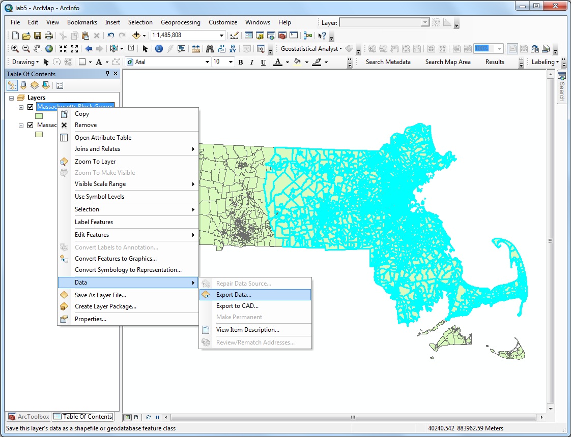
STEP 3: All the Block Groups that intersect with Essex, Middlesex, Worcester, Suffolk, Plymouth, Norfolk, Bristol, and Branstable should now be highlighted. You are ready to create a new file based on these selected features (right click the layer--"Massachusetts Block Groups" and then click ArcMap's Data > Export Data tool). Call this new layer b_blkgrp.shp, save it to your working directory and add this layer into ArcMAP. Follow the same process to export a shapefile of the selected counties. As usual, these operations will be much faster if your 'working directory' is a truly local drive.

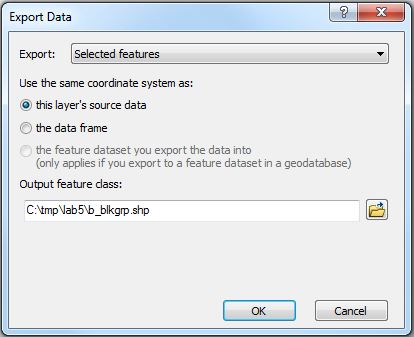Fig. 1. Export to a new shape file

STEP 4:

In your data frame, remove the two layers with data for all of Massachusetts for block groups and counties. We no longer need these files and their size could affect processing speed. From this point you will only need to use the b_blkgrp.shp layer. Be sure to save your ArcMap session at this point.

Part IV: Working with ACS Data : Finding The Variables

These instructions explain how to identify a particular ACS variable of interest and join the tabular ACS data to a geographic boundary file. In the following steps, we will first identify which ACS table and fields we are interested in. Second, we will import the table into access to do some basic data processing. Lastly, we will join the tabular data to a geographic boundary file.

STEP 1: Determining the desired ACS variable.

Open the ACS 2013, 5-year, Appendices (.xls) and search the string/key words "means of transportation to work". Clicking through, we will find "B08301. MEANS OF TRANSPORTATION TO WORK". There are 20 columns in the B08301 matrix. Its Summary File sequence is 0028 and the starting and ending Summary File positions are 157 and 177. Lets take a look at exactly what data is in this table. Open the B08301 table shell (you can download ACS table shells from the Census Bureau's FTP site). The first row of table B08301 reports the total count of workers 16 years of age and over (that is the universe for B08301), and the third row reports the count of workers who drove to work alone. So the we need the first and third rows of this table for this lab.

STEP 2: Locating the table of interest in the ACS geodatabase.

Lets take a look at the metadata for the ACS block group geodatabase. The data is structured with the table name first, followed by either an "e" or an "m", followed by an integer. The "e" and "m" indicate whether the attribute is an estimate or a margin of error (unlike with the Decennial Census, the ACS estimates include a margin of error). The last integer is the row number in the table. Lets make sure that this is right? Use "find" to to search for B08301. As expected, B08301e1 is "MEANS OF TRANSPORTATION TO WORK: Total: Workers 16 years and over -- (Estimate)" and B08301e3 is "MEANS OF TRANSPORTATION TO WORK: Car, truck, or van: Drove alone: Workers 16 years and over -- (Estimate)"

Next, click the "add data" button on you map. Navigate to the ACS geodatabase. Click the geodatabase to look at the files inside it. There are a bunch of tables named by the type of data that they contain and one geographic boundary file. Looking at the table names, it seems like the table that has the B08301 data would be X08_COMMUTING. Add that table to the map.

Lets look inside the table X08. First, make sure that "List by Source" is the selected view type in your table of contents. If you have "List by Drawing Order" selected you will not see the table in the table of contents. Next, right click the table and select "Open". We want to make sure that the table contains the fields B08301e1 and B08301e3. Does it?

STEP 3: Importing the table of interest into MS-Access.

ArcGIS can use two types of geodatabases, a file geodatabase or a personal geodatabase. There are several differences between the two geodatabase type, but the one that we need to note is that MS-Access can open tables directly in a personal geodatabase but not a file geodatabase. There are two ways we can determine what type of geodatabase the ACS geodatabase is. We could look at the site where we downloaded it from to see if the tell us or we could right click on the ACS geodatabase in ArcCatolog toolbar in ArcMap (or the standalone ArcCatalog program), select properties, and look at the "General" tab.

Since the ACS geodatabase is a file geodatabse we will need to export the table X08_COMMUTING as a file type that can be imported into MS-Access (i.e. mdb., .txt, .xls, etc.). To make things run smoothly, we've added a .xls table that is an abreviated version of table X08 to ./data/lab5_ACS_09_13. The file is called X08_Short.xls. To save a bit of time, we are going to have you import X08Short.xlsinto MS-Access instead of table X08.

How did we create X08Short.xls? We created a copy of table X08 in the geodatabase. Then, using the ArcGIS delete field tool we deleted the fields from X08 that we did not need for this lab (i.e. we got rid of all ACS data fields that we did not need but kept B08301e1, B08301e3, and GEOID). We then exported the shortened table to xls in ArcGIS.

Open MS-Access and open lab5_ma.mdb.

Select the external data tab. Next, click the "Excel" option.

A pop-up window will appear. Navigate to X08Short.xls and import the table.

STEP 4: Build a table containing the percentage of workers who drive alone to work for and the community type of each block group in Metro Boston.

Open the table you just imported into MS-ACCESS. The table has three fields. The first field, GEOID, is the field that lets us join the tabular data to our block group geometry file. SInce we already figured out what ACS field names mean what, we know that the second field, B08301e1, is a count of all workers 16 and the third field, B08301e3, is a count of workers who drove to work alone.

We want to calculate the percent of workers who drove to work alone. We have a hunch that the type of community that a block group is located in might impact the percentage of people who drive to work alone. The Metropolitan Area Planning Commission (MAPC) has categorized communities/towns in the Metro-Boston as being "inner core", "regional urban centers", "maturing suburbs", "developing suburbs", or "rural towns". They have released a table with the names of towns and the category of the town. We've already loaded this table into ./data/lab5_ACS_09_13 for you as Comtype. We've also loaded a "cross-walk" that lists what town every block group in Massachusetts is located in, BGLookUp.

Before we start working with these table, lets take a quick look at them. Open X08Short.DBF. The table has 4,985 records. Why? Open ComType. How many records does it have? Open BGLookUp. The table has 4,981 records. Why (hint: when we created BGLookUp>, we excluded "off shore" block groups)?

To calculate the percentage of workers who drove alone to work for and associate the community type data with each block group, we are going to build two queries. As in many things, there are several different ways one could accomplish this task. One way would be to do it in ArcGIS. You could also do it in Excel. We are going to show you how to do it in MS-Access. When you are doing this type of task in the future, you will have to determine what method works best for your particular project.

We are now going to build our first query. Click the "Create" tab in the main menu and the "Query Design" to get a screen like the following:

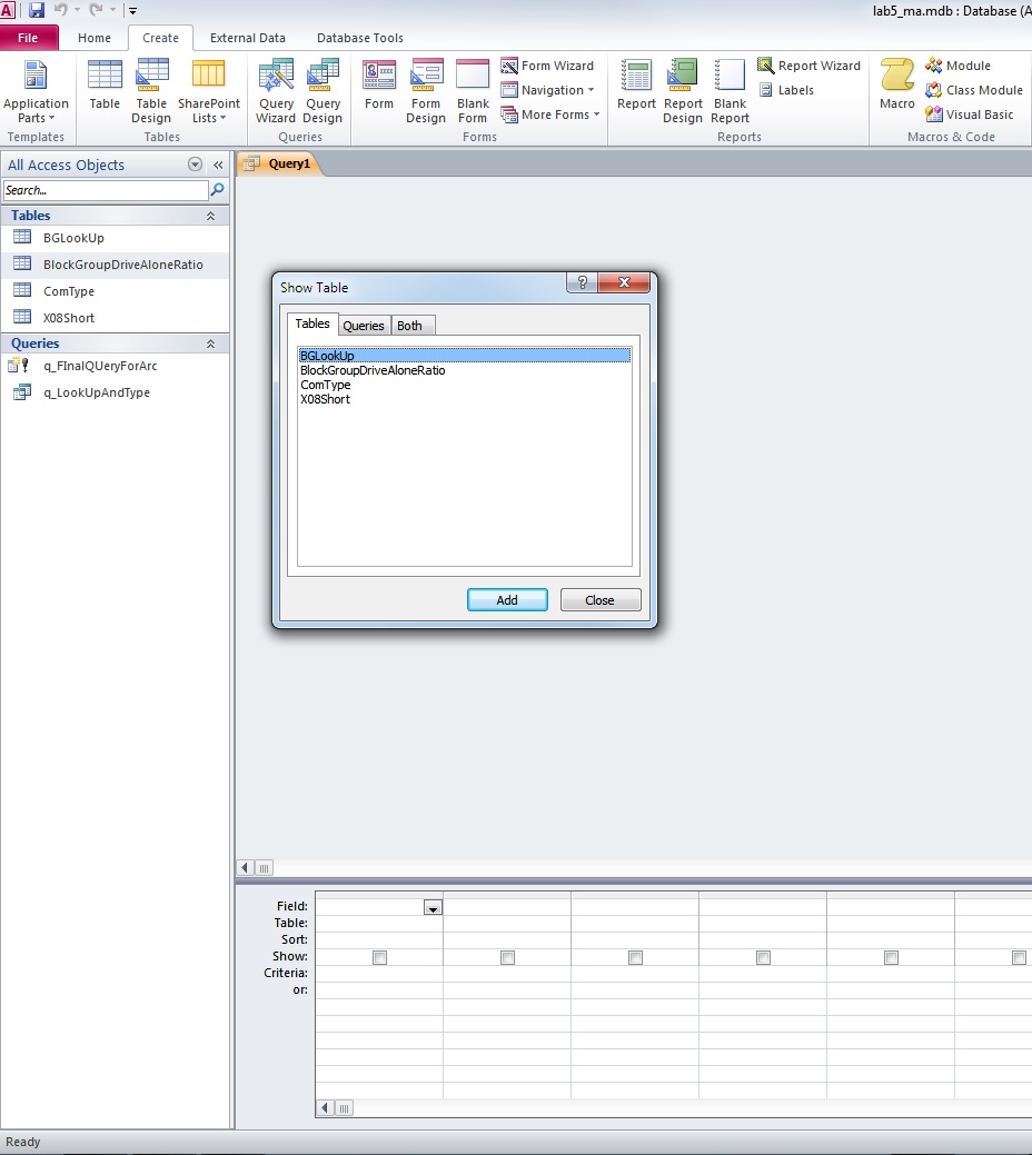
Select tables BGLookUp and ComType. Add them in and close the "Show Table" window.

Now join the two tables by dragging and dropping the Town field in the BGLookUp table onto the COMMUNITY field in the ComType. (Do you understand what this does?) The query window will look something like the following.

Add all the fields in the BGLookUp table to the query by double-clicking the "*". Add the Community Type field in the ComType table by double-clicking the field. Your query window will look something like the following.

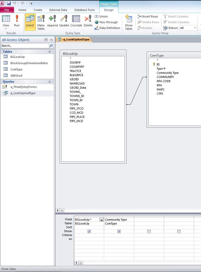
Click the "Run" button on the design tab's ribbon. Right-click the query tab and select "save". Call the query q_LookUpAndType.

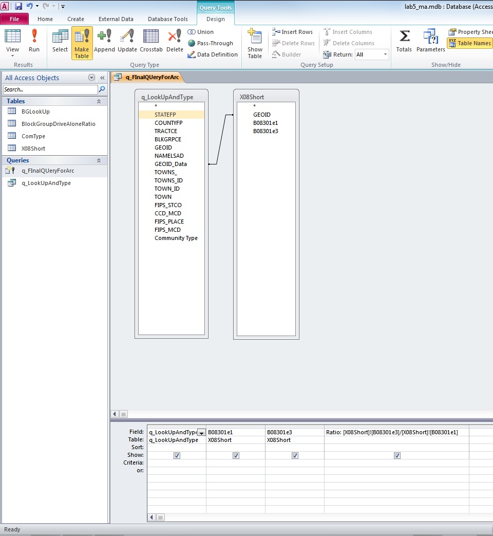
We are now going to to create a query that joins the ACS data in XOShort and calculates the percentage of workers who drive alone to work. Click the "Create" tab in the main menu and the "Query Design".

Select the query we just made, q_LookUpAndType and XOShort. Add them in and close the "Show Table" window.

Now join the query and the table by dragging and dropping the GEOID_Data field in the q_LookUpAndType query onto the GEOID field in the XOShort table. Do you understand what this does?

Add all the fields in the q_LookUpAndType query to the query by double-clicking the "*". Add the B08301e1 and B08301e1 field in the XOShort. Now we are going to create a field in the query that calculates the percentage of workers who drive to work alone

In one empty column at the bottom of the query design view, right-click and choose "Build". In the expression builder that pops up, type in "Ratio: [X08Short]![B08301e3] / [X08Short]![B08301e1]" and click OK. Do you understand what this expression does? What would be wrong with entering "Ratio: [X08Short]![B08301e1] / [X08Short]![B08301e3]"? How about "Ratio [X08Short]![B08301e3] / [X08Short]![B08301e1]"? Your Query window will look something like the following.

You can preview your table by clicking "Run!" under the Query Menu. You should have 4978 rows in the resulting table. You can save this query (via file save) and MS-Access will save the SQL instructions that describe your query (rather than the output table itself). However, ArcGIS sometimes has problems with data types when importing queries from Access. In order to clarify data types, we will use this query to create a new Access table. Switch back to the 'Design View' for the query. (Click the 'View' button on the left of the main menu. Click the arrow below 'View' to see the choices.) In the 'Query Type' section of the main menu, choose "Make-table query", enter the table name "BlockGroupDriveAloneRatio" and click OK. At this point you have identified the name of the table you would like to save - but you have not yet created the table!

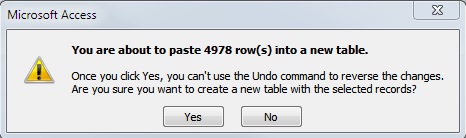
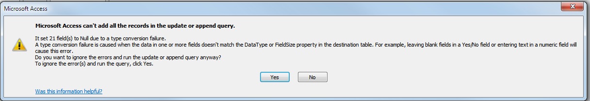
Under the Query Tools (Design) menu, click "Run!". Two message windows will pop up as shown below. Click Yes to confirm both. The second message window is complaining because some of the selected block groups have no population aged 16 and over, in which case the percentage formula is trying to divide by zero. You could avoid the error message by further restricting the query to select only those block groups for which B08301e1 is 0. [BEWARE: MS-Access will insert a zero for any block group without workers aged 16 and over, and it will properly calculate the fraction for the rest. However, when using ArcMap to do a similar calculation, ArcMap will stop processing records as soon as it encounters a 'divide by zero' error. All the remaining rows are then likely to contain a zero value. So it is better practice to do calculations involving division only on those rows for which the denominator is never zero.]

Turn in a screen shot of your BlockGroupDriveAloneRatio table in Access with a dozen or so rows visible along with the columns you used to calculate the ratio, the column with the calculated ratio, the the column with the unique geographic identifier, and the status line at the bottom of the MS-Access table that shows the total number of rows in the table.

Part V: Join the BlockGroupDriveAloneRatio table from to the Block Group Layer in ArcMAP and Create a Layout.

Next, we want to add into ArcMap the table BlockGroupDriveAloneRatio from the MS Access database.ArcMap will recognize MS-Access database files (ending in *.mdb) in the same was that you can 'Add' shapefile to ArcMap by finding them in the file system. So, we add the table just as we would add a shapefile by navigating to the file directory where we stored lab5_ma.mdb. (It is also possible to define a new OLE database connection (from within ArcCatalog or ArcMap) using the Microsoft Jet driver in order to import MS-Access tables into ArcMap. That method will save MS-Access queries as well as tables but can have data type conversion problems). If you cannot see your MS-Access database, then it is probably not in the .mdb format. You will need to save it as in an .mdb format.

After adding your BlockGroupDriveAloneRatio table, join it to the Boston Block Group layer using the field GEOID_Data in the BlockGroupDriveAloneRatio table and the field GEOID_Data from the Boston Block Group attribute table.

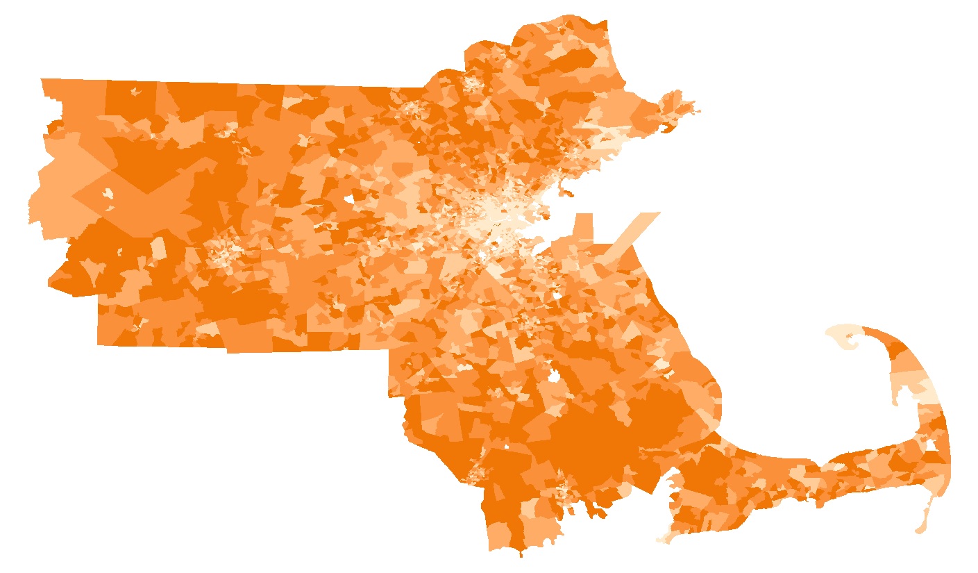
Make a thematic map showing the ratio of drive-alone workers by block group using the "Ratio" field in the table (Choose a reasonable symbology method and explain your choice). The map should be similar to the following one

As always, include the appropriate cartographic elements (scale, legend, title, author & date, source(s), north arrow) in your map and create a layout. In an annotation section, or on a separate page, write a few sentences that interpret your results (e.g., are the percentages driving alone surprisingly large or small; which classification method did you choose and why, do you see any pattern regarding block groups near and far from metropolitan centers or transportation corridors?) Do any of the MassGIS or ESRI web services help interpret the map by providing useful background or overlay data?

Export the final layout into a ".pdf" file, save it in your network locker and submit your map and explanatory text to us via Stellar as one file.

Part VI: Getting data from MIT Geodata Repository (Optional)

For this exercise, both the attribute data will come from the detailed census tabulations that are available online and were discussed in last week's lecture. The census block group geographies are also available online but we have provided a copy in the class locker (as discussed in Part I). The MIT Libraries maintains a GeoWeb site that allows these and many other geospatial data sets to be downloaded. You are not required to use this online geospatial data repository for this census lab exercise, but the GeoWeb is likely to be a useful data resource for your individual project work later in the semester. You may want to check out the GeoWeb now and get comfortable with the interface and resources that it offers.

The MIT Library's GeoWeb is here and the homepage for all the MIT Library GIS Services is here: here.

In order to use the MIT Geodata Repository to download boundary files directly into ArcMap, you will need to register with the MIT Libraries and activate the MIT GeoData Search Tool extension to ArcGIS. The Search Tool extension is already available for use by the Lab machines, so you will only need to install it on your personal machine. You can download the tool from IS&T here. The library also provides some information about the tool.

For this optional lab exercise, you can use the GeoData Search Tool to download Massachusetts Block Group 2000 and Massachusetts County Boundaries 1991. You will need an account with the Library and you will need an MIT web certificate to register for the account. At this point, you should create your account either by following the instructions in the above link, or by clicking on the registration button of the Search Tool's login window. When registering use your MIT Athena (kerberos) ID but we suggest that you choose a different password since your Athena account is your most personal and important MIT account and you should not repeat its password for other accounts.

Open ArcMap and make sure that the MIT Geodata Repository tool is available. Even though the MITGeodataTool.dll is installed, we may still have to tell ArcMap to include it in our own personal ToolBar. If you do not see the MIT GeodataRepository tool, then right click in the toolbars areas of the ArcMap window and choose "MIT Geodata Repository Toolbar" in the context menu. You may also need to click the "MIT GeoData Repository" toolbar after choosing View/Toolbar in order for the toolbar to become visible. This toolbar looks something like this: (The version installed on lab machines may differ slightly from the images shown here.)

When you first click any of the items on the toolbar, you will be prompted to login via a screen like this:

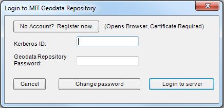
You need to register for an account in MIT Geodata Repository before you can use it. Click on "No Account? Register Now" and follow the instructions in the pop up Internet Explorer window to create a user account if you have not already registered. [Note also, that you must click 'Login to server' rather then just hit 'enter' after typing your password!!]

There are several ways to locate the 2000 Census Block Group boundary files. One way is to use the MIT Library's GeoWeb in a browser (as explained in Lab Exercise #1) and choose 'save link to this map' once you have found the dataset. Then you can click 'Data from Geoweb' on the Geodata Repository toolbar and then (once you are logged in) you can paste the link into the window that opens up. The link will be used by ArcMap to pull the census block group boundary files directly into ArcMap from the Geodata Repository.

Alternatively, you can click on the "Search Metadata " option on the Geodata Repository toolbar and browse the data in the Repository. Once you have logged in, you will see this screen:

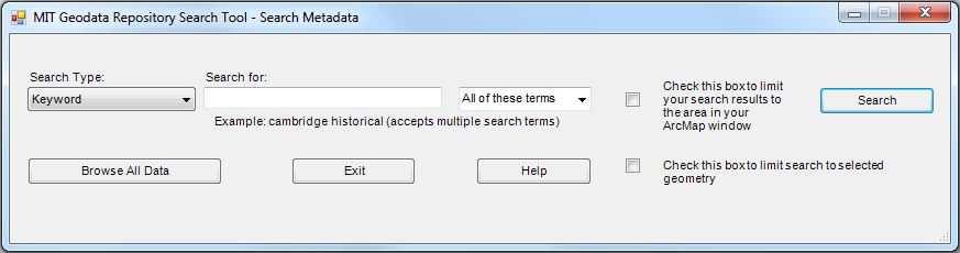
Choose "Keyword" for the search type and search for "Massachusetts block group". Click on "Search" to get a search result that includes the following:

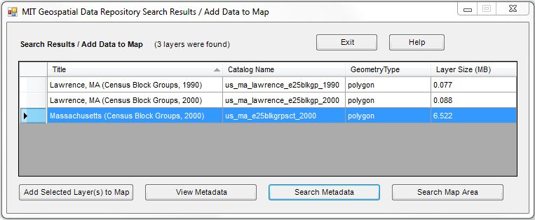
Note: Your results may look a little different from the screenshot since the MIT Libraries have updated some of the names of their datasets. For this lab exercise, we used two layers from the MIT GeoWeb:

• 2000 Mass Census block groups: SDE_DATA_US_MA_E25BLKGRPSCT_2000
• 2000 Mass Country boundaries: SDE_DATA_US_MA_E25COUNTIESCT_2000.

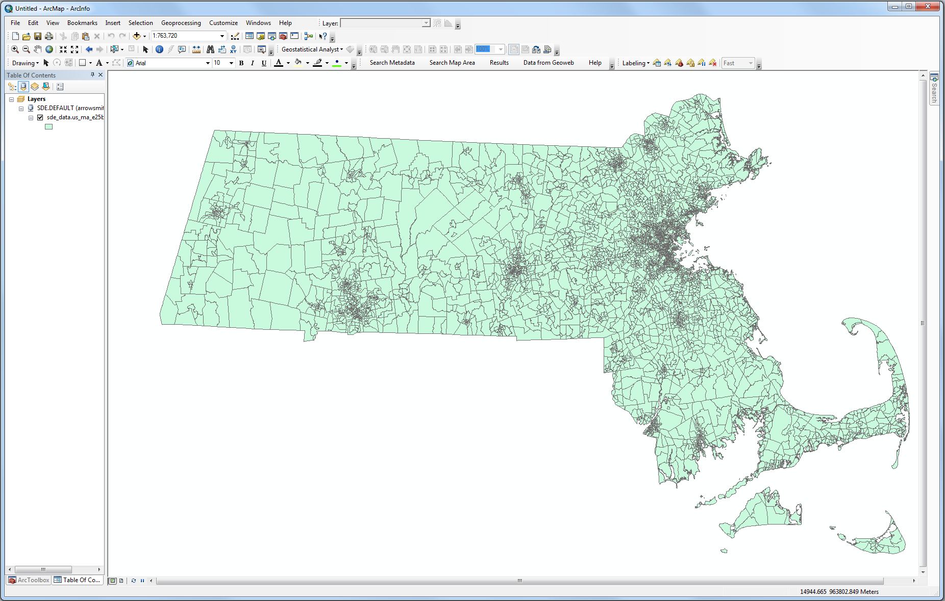
Click "Add Selected Layer to Map". It will take a while for the layer to be added from the MIT Geodata Repository server. The ArcMap window now should look like:

Part VII. Assignment

Please submit to Stellar your lab exercise including your MS-Access screen shot from Part IV and your ArcMap layout from Part VI, plus your text discussing your results. You should submit ONE file that includes all the parts of the lab assignment. The assignment is due on Monday, March 16th, 2015.

Developed by Thomas H. Grayson and Joe Ferreira, 1998.
Modified 2000-2015 by Anne Kinsella Thompson, Thomas H. Grayson, Sarah Williams, Jeeseong Chung, Jinhua Zhao, Xiongjiu Liao, Mi Diao, Lulu Xue, Shan Jiang, Jingsi Xu Eric Schultheis and Joe Ferreira. Last Modified by [schulthe] on 25 February, 2015.

Back to the 11.188 Home Page. Back to the CRON Home Page.