Review a few points from last lecture

• Creating new geometry
  • create empty shapefile in ArcCatalog, then add geometry via ArcEdit
• Advanced raster analysis steps
  • Have you set appropriate Spatial-Analyst options: grid cell size, extents, mask, map units, coordinate system
  • Do you have a sense of available tools beyond the basics: map algebra, zonal statistics, surface analysis and smoothing (contours, hillshade, interpolation,...), and use of model builder
• Workspace
  • By default, ArcMap on WinAthena PCs will use: C:\Documents and Settings\jf\Local Settings\Temp\
  • This is a network drive - on your H:\ locker - and is an AFS file system (Andrew File System)
  • Hence it is slow and prone to timeouts compared with a local drive
  • For most class exercises, using a network drive is fine
  • But for project work, where you may have larger or more complex shapefiles and data, you may have problems
  • When working with larger layers or complex operations (such as intersections), consider
    • Saving intermediate files locally
    • Setting your 'current workspace' and your 'scratch workspace' to a local drive
      • Right-click ArcToolbox/Environment-settings/General Settings
      • Specify local, writeable sub-directories for current and scratch workspaces
      • Before logging out, be sure to use ArcCatalog to copy anything you want to save to a network drive
      • Beware that saved ArcMap documents may not find layers that have been moved - look at properties and 'set data source'
• Raster Analysis example
  • Review setting up the grid size, extent, and mask options
  • Add a shapefile (that we created last time using ArcEdit) with one or two new polygons over part of Cambridge (which we will call our zones)
  • Use zonal statistics to compute the mean of housing+land value for portion of Cambridge within each polygon in the newly created 'zonal' shapefile
    • Sounds easy but can be tricky because of one of the ArcGIS 'gotchas'. Handling raster layer attribute tables and converting between floating point and integer (think of classification not continuous measurement) is tricky. Raster (grid) layers do not have the same kind of attribute tables as vector layers (such as shapefiles). If the grid cell values are integers , you can open the attribute table (called a 'value attribute table') for the grid layer and it will have one row per unique value together with a count of the number of grid cells containing that value. However, if the grid cell values are floating points (as is the case for the interpolated sales89 grid cell values), you cannot open the attribute table (even though you can generate a thematic map of the values). This is practical since a 1000x1000 grid cell matrix implies 1 million cells whose values, if floating point numbers might all be unique.
    • Using the 'zonal statistics' tool can produce a new raster grid layer with grid cells cookie cut throughout each polygon in the new shapefile and with grid cell values (floating points) that are the same for each grid cell inside each polygon (in the new shapefile) and are equal to the average (or min, max, standard deviation, etc.) of the interpolated house+land value grid cells inside each polygon. It is analogous to the 'summary statistics' command we say earlier but the grouping is based on location (within a new polygon 'zone') instead of based on common values in an attribute table.
    • The new output layer created by 'zonal statistics' does not have an attribute table (since the cell value are floating points) but you can map it thematically (one shade for the average value within each zone)
    • Use the 'zonal statistics as table' tool to create a new table with one row per polygon (in the new zone shapefile) and with columns (mean, min, max, ... values) that are computed based on all the interpolated house+land values for the grid cells in each zone. So the values in the 'Mean' column are the same as the thematically mapped for the 'zonal statistics' result above. You can join this new table to the new polygon shapefile that represented the original zones. Try it.
  • Scan other spatial analyst tools in ArcToolbox
• Using OGC-complaint web mapping services (i.e., WMS servers)
  • ArcGIS version 9.2 has trouble with WMS servers such as at MassGIS - ArcGIS version 9.3 is better but not in the lab.
  • Illustrate use in Google Earth
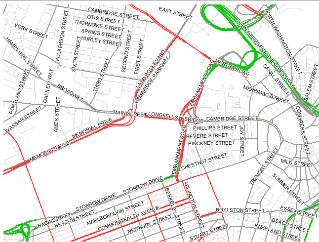
    • Recall URL that overlays streets and street names using the MassGIS services: (Try this URL in a browser): Image A:
      • http://maps.massgis.state.ma.us/mapaccess/main.jsp?dpi=120&request=GetMap&layers=MHD+Roads&styles=Class&srs=EPSG:26986&bbox=233500,900000,236500,902500&width=640&height=480&format=image/png&service=wms  
    • We can put (almost) the same URL into Google Earth in order to overlay street names when we are looking at Massachusetts areas
      • Add &transparent=true at end of URL so WMS map image is transparent (except for streets and street names)
      • Change EPSG (coordinate system ID) to 4326 (WGS84, lat/lon coordinates)
      • Change the orginal bounding box to be appropriate lat/lon: &bbox=-71.1,42.35,-71.0,42.37
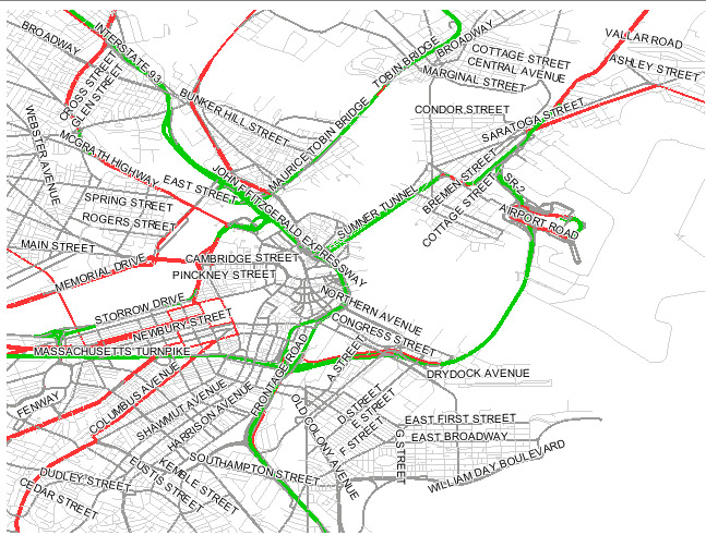
      • The resulting URL is: Image B:
      • http://maps.massgis.state.ma.us/mapaccess/main.jsp?dpi=120&request=GetMap&layers=MHD+Roads&styles=Class&srs=EPSG:4326&bbox=-71.1,42.35,-71.0,42.37&width=640&height=480&format=image/png&service=wms&transparent=true
    • After launching Google Earth, choose Add/Image-overlay and use the following parameters:
      • Name: MassGIS-street-map
      • Link: (paste in the above (Image B) URL)
      • Refresh-tab: set "when" to be "after camera stops"
      • Here are the images returned as Image A and Image B from the MassGIS server:

  Image A: MassGIS Roads Overlay (in State Plane Coordinates)	Image B: MassGIS Roads Overlay (in lat/lon)

Network Analysis (not covered on test)

• Encoding proximity using a network (or graph) model, facilitates certain types of connectivity analyses
  • Find shortest path along streets from Point A to Point B
  • Find shortest path through N cities (Traveling Salesman problem)
  • How far can you get in 30 minutes
• Many transportation analyses use network data models
• Many hydological analyses use network data models (runoff, flow, ...)