| 11.520: A Workshop on Geographic Information Systems |
| 11.188: Urban Planning and Social Science Laboratory |
Lab Exercise 5:
Working with 2000 Census Data & MIT Geodata Repository
Due October 19, 2009
In this exercise you will use the Census STF3 files to create a thematic map indicating the percentage of workers in block groups in and around Middlesex County who drive alone to their jobs. The data about mode choice for workers comes from the 2000 US Census data and the boundary files for Mass census block groups comes from the MIT Geodata Repository maintained by the MIT Libraries. (The MIT Geodata Repository provides online access to an ArcSDE spatial database engine containing many large, useful GIS datasets.)
In order to develop this map, you will have to create a table that contains the percentage of workers who drive alone to work (by car, truck, or van) for each block group in Boston Metropolitan Area. But the raw census data provide counts of the number of workers within each block group that use each transportation mode to get to work. Unlike the simple example (involving median earnings) shown in class, computing this percentage will require normalizing the census counts. (Here's a link to some additional discussion about when and how to normalize the data.)
Useful Resources :
The in-lab discussion notes are here: Lab #5 notes but they do not contain anything beyond what is in this lab exercise.
We are going to use two geographical layers from the MIT Geodata Repository--Massachusetts Block Group 2000 and Massachusetts County Boundaries 1991. The MIT Geodata Repository is one of the GIS services offered by the MIT Libraries. See their GIS homepage for more info: http://libraries.mit.edu/gis/index.html The MIT Geodata Repository description is here: http://libraries.mit.edu/gis/data/repository.html You will need the instructions from this site if you want to load the toolbar onto your own ArcGIS installation. The lab machines already have the MITGeodataTool.dll installed.
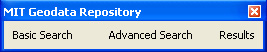
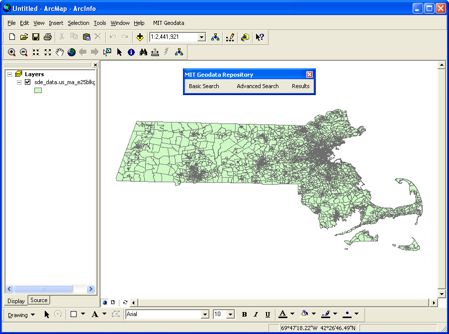
Even though the MITGeodataTool.dll is installed, we may still have to tell ArcMap to include it in our ToolBar. If you do not see the MIT GeodataRepository tool, then right click in the toolbars areas of the ArcMap window and choose "MIT Geodata Repository Toolbar" in the context menu. (The latest version may have more buttons than are shown here.)
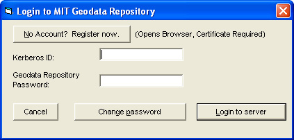
Click on "Advanced Search", and a Login window should show up as follows,
You need to register for an account in MIT Geodata Repository before you can use it. Click on "No Account? Register Now" and follow the instructions in the pop up Internet Explorer window to create a user account.
After the registation, log in using your Kerberos ID and the Geodata Repository Password you choose in the registration and click on "Login to server".
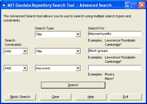
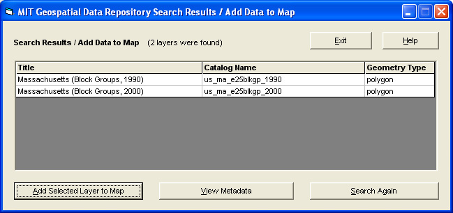
In the Advanced Search window as above, choose "Title" and Search for "Massachusetts" and "Block groups". Click on "Search" to get the search result as follows,
Click on the second row (Block Groups 2000) and click "Add Selected Layer to Map". It will take a while for the layer to be added from the MIT Geodata Repository server. The ArcMap window now should look like,
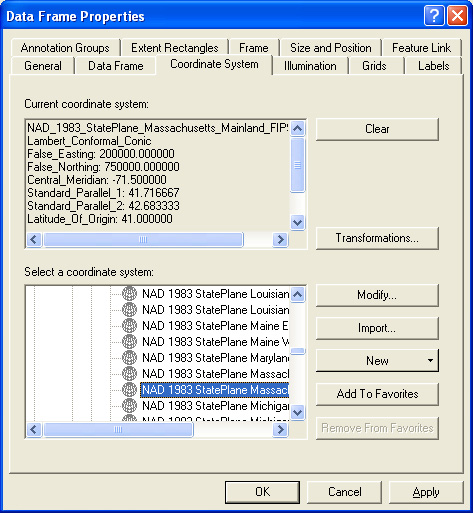
Depending upon which shapefile you downloaded, the Block Groups layer may be displayed in geographic coordinates (lat/lon) instead of the desired correct projection (Mass State Plane). If necessary, change the projection to "State Plane / NAD 1983 / NAD_1983_StatePlane_Massachusetts_Mainland_FIPS_2001" from the "Coordinate System" tab in the Data Frame Property window. In “Select a coordinate system” window, expand “Predefined”, then “Projected Coordinate Systems”, followed by “State Plane”, “DAD 1993”, and “NAD 1983 StatePlane Massachusetts_Mainland_FIPS_2001”.
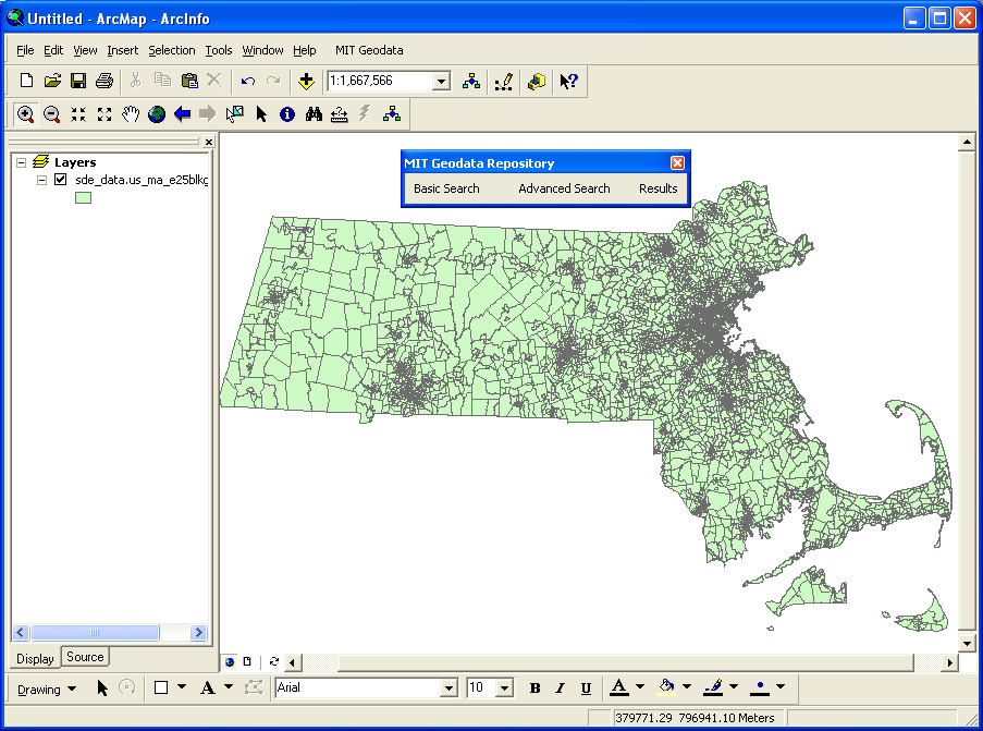
After the correct coordinate system is specified, ArcMap will redisplay the Block Groups layer as follows. (Note that Mass is not as 'squished' as it was in the lat/lon view. Do you remember [from the earlier lecture on coordinate systems and projections] why this is the case?)
Add in the "Massachusetts County Boundaries 1991" layer from MIT Geodata Repository in the same way as we add the "Block Groups" layer.
In order to work with a smaller file, we want to create a new Shapefile that represents the Block Groups that fall within major Boston area counties (Essex, Middlesex, Worcester, Suffolk, Plymouth, Norfolk, Bristol, and Branstable). We can select these block groups using the Select By Location tool in ArcMAP.
STEP 1.In the Massachusetts County Boundaries layer, select
Essex, Middlesex, Worcester, Suffolk, Plymouth, Norfolk, Bristol, and Branstable
counties. If you are familiar with counties in Massachusetts, you can simply
use the graphical selection tools ![]() to select the eight counties. If you aren't, use the Selection > Select By
Attribute tool to select these eight counties by name from the attribute table of the county layer.
to select the eight counties. If you aren't, use the Selection > Select By
Attribute tool to select these eight counties by name from the attribute table of the county layer.
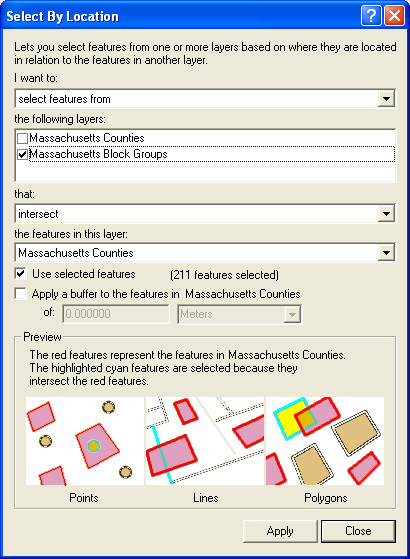
STEP 2. With the counties selected you are ready to use the Select By Location tool. This tool works on the currently active theme, so you will need to make the Massachusetts Block Groups 2000 layer is active. Go to the Selection menu and select Select By Location.When the dialog window appears, choose to select features from your active layer (Massachusetts Block Groups 2000) that Intersect with the selected features of the U.S. Counties layer. Refer to the lab 3 for how to use the Select By Location tool.
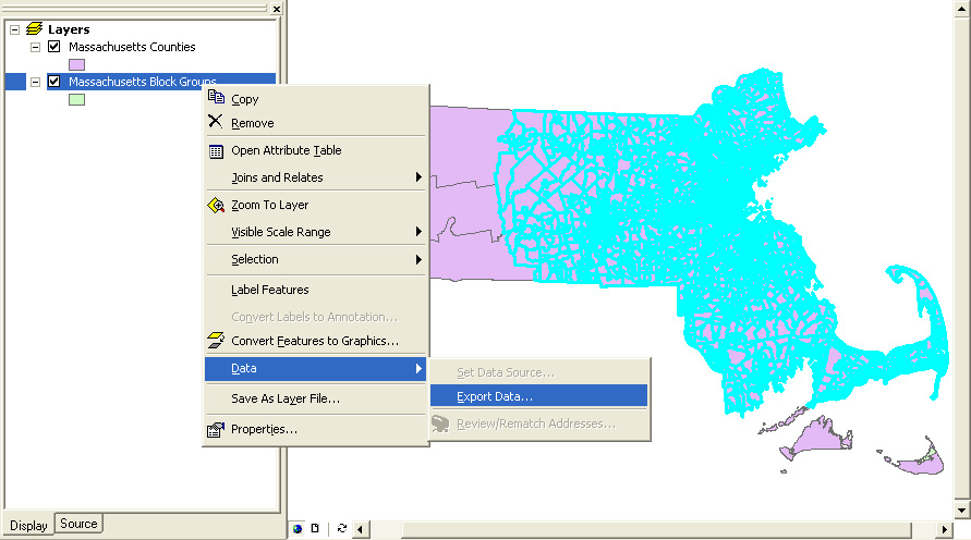
STEP 3: All the Block Groups that intersect with Essex, Middlesex,
Worcester, Suffolk, Plymouth, Norfolk, Bristol, and Branstable should now be
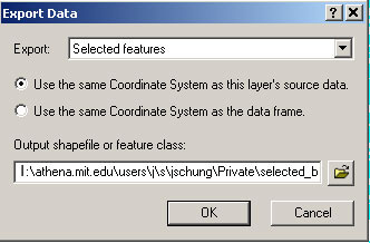
highlighted. You are ready to create a new file based on these selected features
using ArcMap's Data > Export Data tool (Refer the images below). Call
this new layer b_blkgrp.shp, save it to your working directory and add
this layer into ArcMAP.
 |
 |
STEP 4: In your data frame, remove the two layers from MIT Geodata Repository. We no longer need these file and their size could affect processing speed. From this point you will only need to use the b_blkgrp.shp layer.
These instructions explain how to identify a particular census variable of interest and extract it from the freely distributed text files containing the raw SF3 2000 US census data. However, since the processing of the raw text files is cumbersome, we have already imported into MS-Access the raw datasets that contain the tables that you will need. We have retained the full set of instructions in case you want to identify and extract other variables (e.g., for your project later in the semester).
STEP 1: Determining the desired Census variables and the raw text file that includes the desired variables.
Open Summary File 3 : Technical Documentation (.pdf) and search the key word "means of transportation to work". On Page 439, you will find "P30. MEANS OF TRANSPORTATION TO WORK FOR WORKERS 16 YEARS AND OVER [16]". There are 16 columns in the P30 matrix, with variable P030001 reporting the total count of workers 16 years of age and over (that is the universe for P30), and variable P030003 reporting the count of workers who drove to work alone. So the fields P030001 and P030003 are the two columns of our interest for this lab. Next, we have to identify the raw text file which contains the data for these two variables for Massachusetts.
Table 2-2 (File/Table Segmentation) in Chapter 2 of the Summary File 3 : Technical Documentation (.pdf) provides the necessary cross reference information associating the raw text files with particular census variables (specifically, the tables or matrix numbers such as P30). We can see that the file "st00003.uf3" contains the fields from P25 to P37. The P030001 and P030003 of our interest are in this file. For your convenience, we have provided a direct link to the cross-reference table here: 2000 US Census Variable locator. that explains which Census variables appear in which dataset files.
Hence, the raw text files for Massachusetts that we want are "ma00003.uf3" for the P030001 and P030003 variables plus "mageo.uf3" for the geographic identifiers. We have already loaded this raw text file into MS-Access and save the result in M:\data\census2k\lab5_ma.mdb
STEP 2: Copy the access template file, the geographical header file, and the data file "st00003.uf3" to your own working directory I:\11.520\lab5
(Note: The US Census Bureau provides its own detailed explanation of how to import the raw text files for SF3 census data into various databases such as MS-Access. Here is the link: http://www.census.gov/support/SF1ASCII.html. Steps 2 and 3 summarize the way to bring the raw data for Massachusetts into MS-Access. )
The st00003.uf3 file for Massachusetts is ma00003.uf3. All 76 text files, including st00003.uf3, are available (in 'zipped' form) at http://www2.census.gov/census_2000/datasets/Summary_File_3/Massachusetts/. The geographical header file for Massachusetts is mageo.uf3, and is also available at the same online site.
For your convenience, both ma00003.uf3 and mageo.uf3 have been downloaded to our class data locker: M:\data\census2k. This census subdirectory is also visible online as: http://mit.edu/11.520/data/census2k
In order to import these text files into MS-Access, you will also need the MS-Access template file "sf3.mdb." This template file contains variable names, data formats, and the like and is available at http://www.census.gov/support/2000/SF3/. A copy of this sf3.mdb template file has already been downloaded to M:\data\census2k.
In order to manipulate the three files that you need, you should copy them from M:\data\census2k to a local drive on your computer. (You can put them in your network locker - e.g., in I:\11.520\lab5 - but some of the files are large and will not been needed for long.)
STEP 3: Import ma00003.uf3 and mageo.uf3 to sf3.mdb
Before you import the raw text files ma00003.uf3 and mageo.uf3, change their extension name to ".txt" so that MS Access can recognize them as text files. Start MS-Access by double-clicking on your copy of the MS-Aaccess database file sf3.mdb. You will see dozens of tables that are all empty but contain specifications for the structure of each possible census datasset (that is data schema for all the tables).
![]()
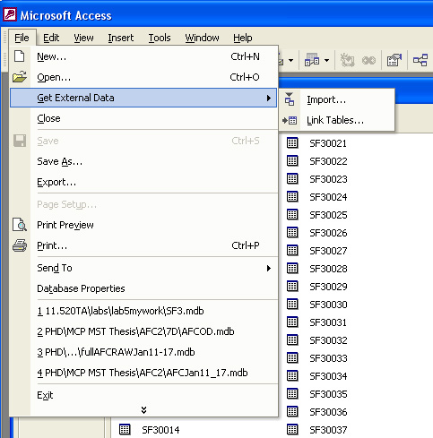
Then click the File-->Get External Data-->Import menu choice as shown below:
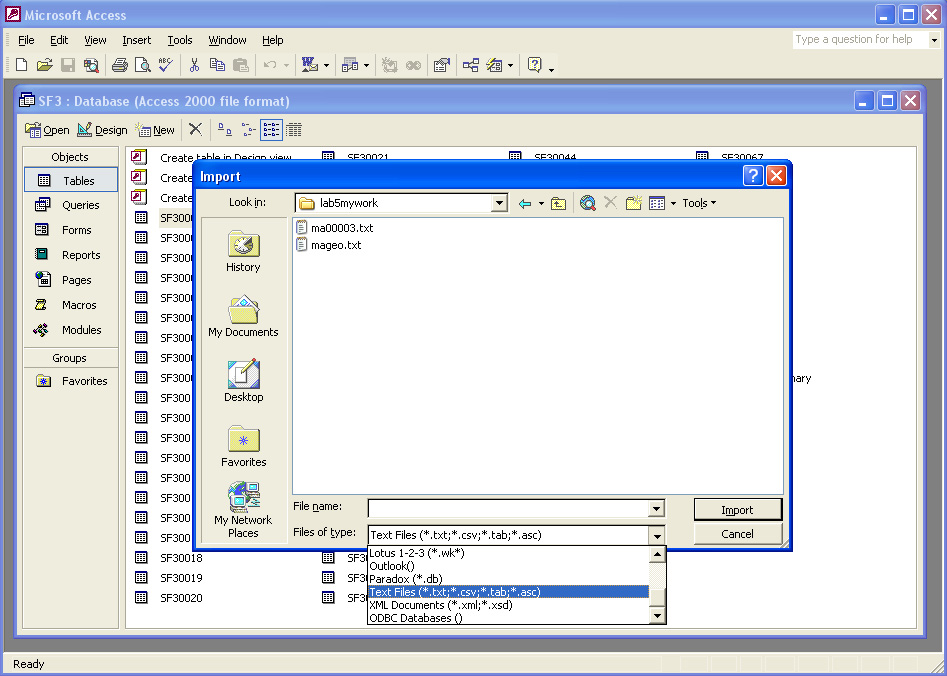
In the Import Window, change the file type to ".txt" files, browse to your working directory and find the "mageo.txt" file.
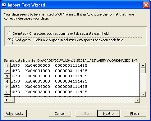
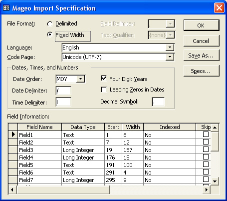
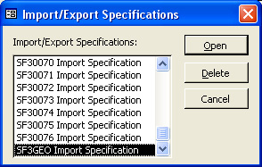
In the Import Text Wizard window, be sure to click "Advanced". After the Import Specification Window pops up, click "Specs...". Scroll to the end to find "SF3GEO Specification" and click Open. Then click OK to return to the Import Text Wizard and click "Finish". The sequences are illustrated as below. (Note that the check boxes on the first few graphic below don't matter since loading in the "SF3GEO Specification" will change the file format type from however it starts out to become 'Delimited' and the code page choice will become '...ASCII'. That is what you want to match the format of the text files.)
Once the "mageo.txt" file is imported, a new table "Mageo" will appear in the MS-Access database control window. You need to import "ma00003.txt" in the same way except using "SF30003 Import Specification".
Note: Since you have now built your own MS-Access database from the raw files, you can now skil to Step 5.
STEP 5: Build a query to construct a table that contains the percentage of workers who drive alone to work for each block group in Metro Boston.
Note: The illustrations below use the MS-Access database created in Steps 2 and 3 and named sf3.mdb. If you are using the lab5_ma.mdb database instead, open up your copy and keep in mind that the illustrations use the sf3.mdb with many more tables than the ma00003 and mageo tables that are in lab5_ma.mdb.
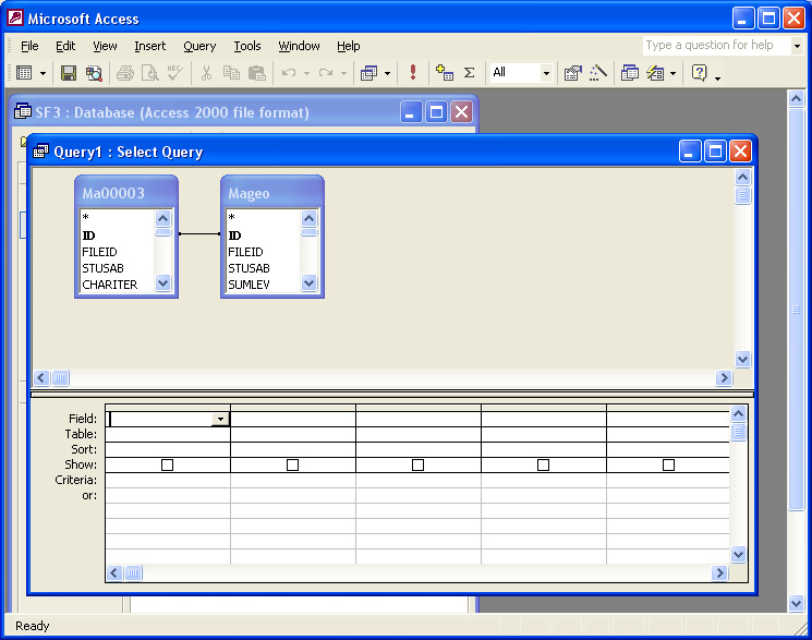
Click on "Queries" in the left pane of MS Access and choose "Create query in design view".
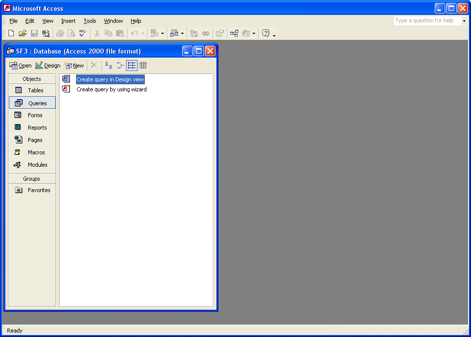
A query design window pops up as below. Select both table "Ma00003" and "Mageo", add them in and close the "Show Table" window.
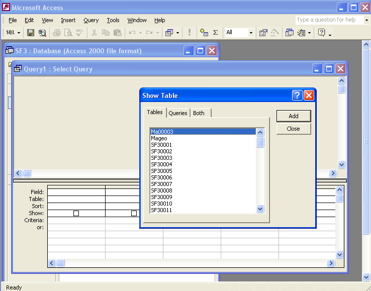
Now the query window looks like the following. (Note: Actually, it is more reliable to join the tables based on 'LOGRECNO,' the census-designated row number, rather than on 'ID,' the row ID in the table.)
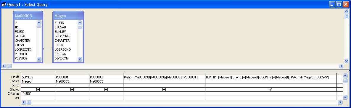
Follow the instructions below to complete the query.
1. Double Click "SUMLEV" in “Mageo” and enter "150" in the Criteria box since the summary level that we want is for block groups (within the simpler geographic nesting hierarchy that does not include 'place').
2. Double Click on P030001 and P030003 in “Ma00003” so that both fields show up in the bottom tables.
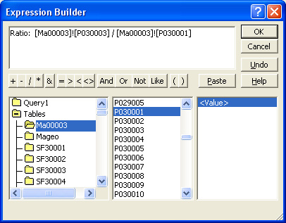
3. Next, we want to define a column that computes the fraction of drivers who drive to work alone. In one empty column of the bottom table, right click and choose "build". In the expression builder that pops up, type in "Ratio: [Ma00003]![P030003] / [Ma00003]![P030001] " and click OK.
4. We also need to construct a geographic identifier that matches the state+county+tract+blockgroup code in our blockgroup map. In another empty column of the bottom table, right click and again choose "build". In the expression builder, type in "BLK_ID: [Mageo]![STATE]+[Mageo]![COUNTY]+[Mageo]![TRACT]+[Mageo]![BLKGRP]" and click OK. (Yes, you can cut-and-paste the formula from this exercise!)
5. Link the two tables via the common field LOGRECNO (which stands for 'logical record number').
The final query design should look like the following: (Actually, add the additional constraint that P030001 > 0 so block groups with no workers are excluded.)
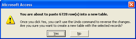
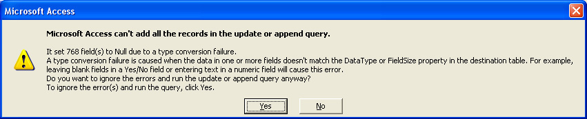
6. You can preview your table by clicking "Run!" under the Query Menu. You can also save the query (via file save). However, ArcGIS sometimes has problems with data types when importing queries from Access. In order to clarify data types, we will use this query to make a new Access table. Under the Query menu, choose "Make-table query", enter the table name "BlockGroupDriveAloneRatio" and click OK.
7. Under the Query menu, click "Run!". Two message windows will pop up as follows, click Yes to confirm both. (Note that, when you use summary level = '150' rather than '090' in the Access query, you will paste 5053 rows rather than 6728 and the second warning message will not appear. Summary level '150' has a single row for each block group. Summary level '090' may have more than one row per block group - it has one row for each unique block group within a 'place'. Since place boundaries sometimes divide block groups into two or more parts, those splits block groups will show up more than once in the summary level = '090' rows.)
STEP 6: Clean up the MS Access database and save the smaller piece that you need.
A new table BlockGroupDriveAloneRatio has been created from the above steps. This table has all the information we need to continue the following lab. In order to save disk space in your own directory, you can export the small table that you just created into another database and then delete your copy of the too-large "sf3.mdb" database by following the steps below.
Use MS-Access to create a new, empty MS-Access database in your working directory and name it, "DriveAloneRatio.mdb." Then, open your local copy of the database named lab5_ma.mdb (and let MS-Access close the new, empty "DriveAloneRatio.mdb" database). In the main database window pane of this MS-Access database, click on "Tables" under 'Objects' along the left side. The BlockGroupDriveAloneRatio table should show at the top of the list. Right click on the table, and choose Export.
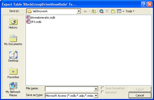
Browse to your working directory, select the database "DriveAloneRatio.mdb" and click Export
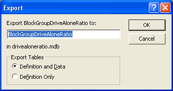
Click OK to confirm the export and then close the MS Access "sf3.mdb" file. In the Windows Explorer, you can check the file size--the sf3.mdb is about 55mb while the DriveAloneRatio.mdb is only 504kb. Open the file DriveAloneRatio.mdb to check if it contains the correct data.Once you confirm that your new, small database is okay, you can delete your copy of the file "sf3.mdb" database to save disk space,. Later in the lab, we only need to use the table in "DriveAloneRatio.mdb".
Next, we want to add into ArcMap the table BlockGroupDriveAloneRatio from the MS Access database DriveAloneRatio.mdb that we just created. ArcMap will recognize MS-Access database files (ending in *.mdb) so we can add the table by just as we would add a shapefile by navigating to the file directory where we stored DriveAloneRatio.mdb. (Remember from class lecture that you can also define a new OLE database connection (from within ArcCatalog or ArcMap) using the Microsoft Jet driver in order to import MS-Access tables into ArcMap. This method will save MS-Access queries as well as tables but can have data type conversion problems).
After adding your BlockGroupDriveAloneRatio table, jJoin it to the Boston Block Group Layer using the field BLK_ID in the BlockGroupDriveAloneRatio table and the field "STFID" from the Boston Block Group Attribute table. [Note, earlier versions of the census block group layer labeled the column 'BLK_KEY'. You want the column containing the state+county+tract+block-group ID that matches the one in you Access table.]
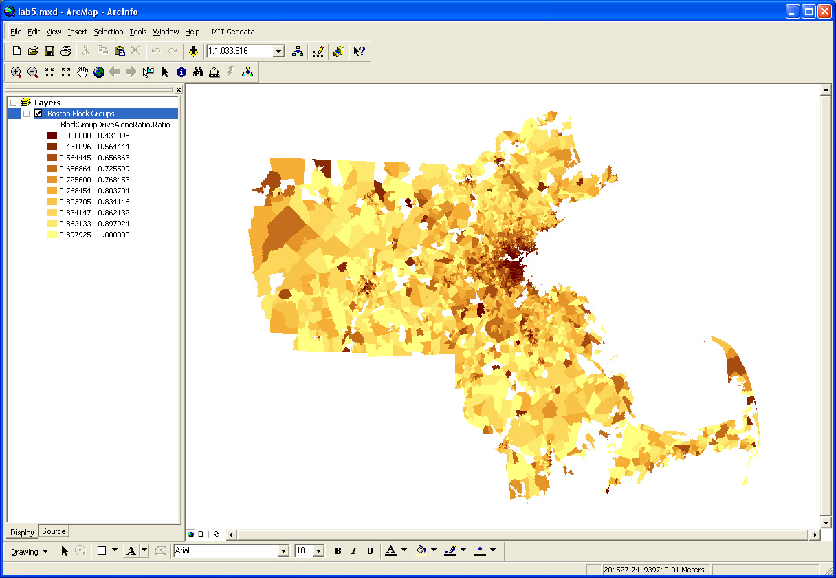
Make a thematic map showing the ratio of drive-alone workers by block group using the "Ratio" field in the table (Choose a reasonable symbology method). The map should be similar to the following one (but with fewer no-data polygons.The map that is shown was generated using summary level = '090' and then ignored those blockgroups that appeared more than once in the table as a result of being split by 'place' boundaries).
As always, include the appropriate cartographic elements in your map and create a layout.
Export the final layout into a ".pdf" file, save it in your www folder and submit it to us via Stellar.
Developed by Thomas H. Grayson and Joe Ferreira, 1998.
Modified 2000-2008 by Anne
Kinsella Thompson, Thomas H. Grayson, Sarah Williams, Jeeseong Chung, Jinhua Zhao, Xiongjiu Liao, Mi Diao, and Joe Ferreira.
Last Modified by Joe Ferreira 12 October 2009.
Back to the 11.520 Home Page. Back to the CRON Home Page.