Lab Exercise 6: Vector Spatial Analysis

• Examine the location patterns of Cambridge stores by using the 'spatial join' tools to tag store location data (bookstores, ice cream shops, record stores) with the demographic characteristics of their neighborhood. (This is a 'point-in-polygon' operation.)
• Create a 1 kilometer buffer around Ames St.
• Estimate the number of young kids living near Ames Street by:
  • Intersecting the Ames St. buffer with the Cambridge blockgroup data
  • Apportioning kids in each blockgroup that is split by the buffer in proportion to the block group area that falls within the buffer
• The in-lab discussion notes are here: Lab #6 notes
  • The notes include the unfinished lecture notes from last Wednesday where we identified which blick groups fell within which city.

Preliminaries

The source for the cambridge_ice_cream.shp, cambridge_bookstores.shp, and cambridge_record_stores.shp layers is the http://www.bigyellow.com/ web site on November 1, 1999. The locations were downloaded from the web page, then geocoded in ArcMap. We'll be exploring address geocoding later in the semester.

Set the map units and display units appropriately: Since the datasets we'll be using are in Mass State Plane coordinates, select View > Data Frame Properties in the menu bar and set the map units to meters and the display units to miles. If you want, you might also change the name to something more informative than "Layers".

Part 1: Point in Polygon Spatial Join and Cluster Analyses

ArcMap can do 'polygons to point' overlay operation using a spatial join. This time, we'll explicitly set up a spatial join between cambridge_bookstores.shp and cambbgrp.shp so that block group attributes can be added to the bookstore table.

Spatial join

• Right-Click the cambridge_bookstores layer in the data frame and select joins and relates > join. The Join Data window will come up.
• Select "Join data from another layer based on spatial location" for the "What do you want to join to this layer" option.
• Choose cambbgrp.shp for the layer to join into the cambridge_bookstores layer.
• Check the "it falls inside" option (Note that the options in the 'join data' window depend on the feature types you are trying to spatially join).
• Specify the name (bookstore_bgrp.shp) of the new file and the location (your working directory) where it is stored.
• Click "OK"

The new shape file you just created (bookstore_bgrp.shp) will be added in your data frame. If you examine the attribute table for bookstore_bgrp.shp you should now see the attributes of cambridge_bookstores and cambbgrp.shp. The "Shape" columns aren't true attributes; they serve as placeholders that link to the geometry of features in the data layer in order to allow us to perform the required spatial joins.

Now we can make a thematic map of cambridge_bookstores.shp using the attributes of cambbgrp.shp. Open the layer property window of bookstore_bgrp.shp to make a "Graduated symbol" map using the "Med_hh_inc" field. You should end up with the bookstore locations sized by the median household income of the block group containing them. To provide additional context for interpreting these locations, create a thematic map of land use using the landuse85.shp layer. This time you can name the file as "bookstore_lu99". Follow the same instructions as in the Explanatory Mapping portion of Lab 2, except that you will use the location of bookstores instead of housing sales. Make sure that the Cambridge TIGER (road) file is also visible in your map.

• For the definition of the land use code, please check the Massgis (Massachusetts Geographic Information Systems) land use definition at
  http://www.state.ma.us/mgis/lus.htm

Take a close look at the pattern of bookstores. Does anything look interesting? Write your observations as requested in the Question 1 of the assignment. Make a layout of your map and submit this as the answer for Question 2.

For extra credit, or just for fun, redo the spatial join, this time tying the block groups to the ice cream stores and the record stores (this requires a spatial join for each of the store layers) and display them on the map too. Do the additional store locations help you to see a pattern?

Part 2: Buffer Analysis

In this part of the lab, you will analyze the demographics of the neighborhood around MIT's biological research facility on Ames Street. You will build on what you learned in the "Simple Buffering" part of Lab 3 to do a more elaborate analysis. In particular, when the buffer boundary cuts through a block group, you will apportion the attributes of that block group based on the fraction of that block group's area that lies inside the buffer. You will use ArcMap to calculate the number of children aged 5 years or under who live within 1 km of the facility.

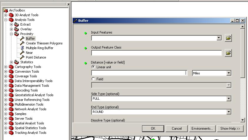
To begin, draw a one kilometer buffer around Ames Street. First you will select Ames Street from the cambtigr coverage and then draw a buffer only around that street. To do this, select the cambtigr layer, then use the Selection > Select by Attributes... menu item to select the arcs where the "FNAME" field is "Ames" and the "FTYPE" field is "St". You may have trouble spotting the arcs you just selected; use the View > Zoom Data > Zoom To Selected Features menu item to help you find them. You should end up with three selected arcs.

Now let's draw a one kilometer buffer around Ames Street. Use the Analysis Tools > Proximity > buffer (see the figure below) in toolbox to start the buffer tool. In the first step, make sure to buffer only the selected features of cambtigr. In the second step, specify a distance of one kilometer. In the third step, tell it to dissolve the barriers between the buffers by selecting "ALL" and save the results in a new layer called amesbuf in your working directory. A new data layer called amesbuf will appear in your data Frame. Now move the amesbuf layer down so that cambtigr and the point layers display above the buffer. You should be able to clearly see the selected arcs in cambtigr at the center of the buffer.

Number of Children within 1 kilometer of Ames Street

Let's take a look at the buffer relative to the block groups. Adjust the display properties of the cambbgrp.shp layer so that it appears only with a thick black border: set the foreground color to transparent and the outline width to 2. Display the layer on top of both cambtigr and amesbuf. You can see that a portion of many block groups falls within the buffer area. We do not want to ignore these split block groups, nor do we want to include all their children in our count. Let's estimate the proportion of each block group that falls within the buffer? The union and intersect operations are good tools for this analysis.

Before using any of these commands let's look at the amesbuf coverage attributes created by the buffer command. When you open the buffer's attribute table, you should see that the buffer command has created a table with one row (since we only produced one buffer polygon) and three columns: the feature ID number (fid), the shape type (polygon) and a column labeled 'ld' that has a value of zero (0). (In this default case, the buffering operation will not generate a field, BufferDis, which contains the buffer distance we specified when we created the buffer).

The union and intersect operations can be used to "overlay" the block group layer with the buffer layer so that the combined layer tags each feature (polygon) with attributes that indicate the original block group and whether the polygon is inside of or outside of the buffer region.

Now let's explore how the union and intersect operations differ. We shall use both operations, union and intersect, to combine all the information attached to the cambbgrp.shp layer with the ones attached to the amesbuf coverage. The union operation computes the geometric intersection of two polygon coverages. All polygons from both coverages will be split at their intersections and preserved in the output coverage. The intersect operation, on the other hand, preserves only those features in the area common to both coverages in the output file. Visually, the difference between these two commands is:

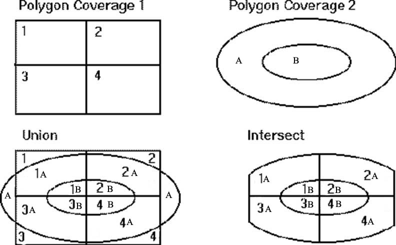
Note that in the Tools > GeoProcessing Wizard, the "input layer" is the layer labeled "Polygon Coverage 1" in the diagram above, and "Polygon Coverage 2" is called the "overlay layer."

Polygon Overlay: Intersect

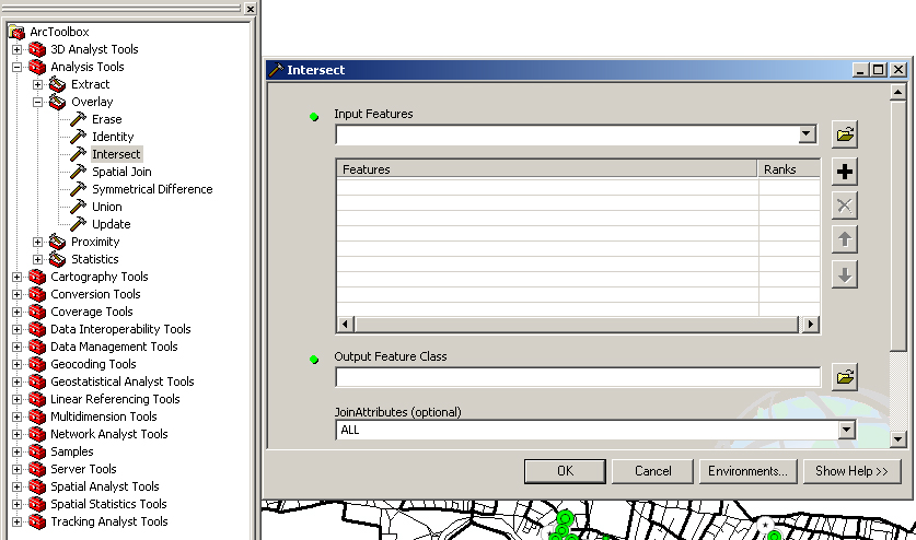
In the Arctoolbox, find the intersect tool (Please see following figure). We will use this intersect option to create a new layer, amesbgbuf_i, that combines both layers. Here is the procedure:

     Procedure:

• Start up the intersect window with the Toolbox>Analysis Tool>Intersect... menu item
• Select "Input features"
• Locate cambbgrp.shp for the "Input features: "
• Locate amesbuf for the "Input features:" (after this step, you will see the above two layers in the "features" portion of the tool)
• Specify the output file [your working directory]/amesbgbuf_i.shp
• Click Finish

Open the attribute table of amesbgbuf, and select the Option > Add Field menu from the bottom of the amesbgbuf_i attribute table and add the following fields to the table:

• Newarea (Type: Float)
• Arearatio (Type: Float)
• Popupto5 (Type : Float)

Click on the "NewArea" field and click the right mouse button. [At this point, you could select 'Calculate Geometry' and compute 'Area,' without need the VBA script.] Select Calculate Values... Check the Advanced box to begin editing VBA script Cut and paste the following VBA statement into the VBA Script text box Dim dblArea as double Dim pArea as IArea Set pArea = [shape] dblArea = pArea.area Type the variable dblArea in the Text box directly under the area field name NewArea = dblArea This VBA code gets the area value for each intersected polygon fragment in amesbgbuf_i from ArcMap's internal data structure. (The internal variable IArea contains this area.) These values are the area within each Cambridge blockgroup that falls within the buffer. You can find the VB code for computing area in the ArcGIS help pages. We want to save these areas in a 'newarea' column since we need the original Area value to compute the portion of each blockgroup within the buffer.

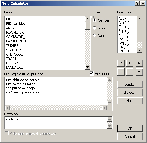Fig.1. Updating Area for a Shape file

Now we are ready to calculate the fraction of each blockgroup that falls within the Ames St. buffer and use that fraction to estimate the number of children living within the buffer. Assuming that the population is distributed evenly throughout each block group polygon in Cambridge, we can estimate the number of children living in the buffer by multiplying each blockgroup's children population count by the computed fraction [Newarea / Area].

First, we'll calculate the ratio of the old to new area. Click on the heading for "Arearatio" and use the Calculate Values... menu item again to set

Arearatio = [Newarea] / [Area]

Popupto5 = ( [Age_lt_1] + [Age_1_2] + [Age_3_4] + [Age_5] ) * [Arearatio]

Polygon Overlay: Union

Repeat all the steps in the "Intersect" section above, with these changes:

• In the Analysis Tools, choose "Union" rather than "Intersect."
• Make the name of the output layer amesbgbuf_u.shp instead of amesbgbuf_i.shp.
• Before you calculate the statistics on amesbgbuf_u.shp, select only those block groups that lie within the buffer. You can identify these because the "FID_amesbu" field (carried over from the buffer attribute table) contains a '0' value for these cases. (The portions of blockgroups that are outside the buffer have a '-1' value.) When you union the layers, all the attributes from both layers are carried over into the new layer. Logically, if a polygon is outsize the buffer, then it is not possible to assign any fields from the buffer layer to that polygon. To compensate, ArcMap will populate these fields in these records with zeroes (for numeric fields). You will need to use the Select by Attribute menu item to restrict the rows to those within the buffer before performing the statistics calculation. If you don't, your answer will be very different than that in the "intersect" part of the exercise.

Refer to the information in the "About Union" box to help you decide what the input and overlay layers are. You should obtain the same numerical results for the child count with either the union or the intersect operation. The geography, however, will look considerably different. For your calculations to work, however, you'll need to keep track of which polygons in the amesbgbuf_u.shp layer were originally inside the buffer; these will be the polygons that have a zero value in the "FID_amesbu" field. Why is this not an issue with the layer you made with the intersect operation? Think about how union is different from intersect even though you can use either as a step toward the same end. Write your answer in the spot for Question 5 in the assignment.

Part 3: Other Spatial Analysis preparation tools (Optional)

- Dissolving features and clipping layers

The above exercises only scratch the surface of spatial analysis tools in ArcGIS. We don't have time for more required exercises. This optional exercise focuses on two common operations:

1. DISSOLVE - suppose we have a census block group map and we wish to create a census tract map. We can use the 'dissolve' tool to eliminate the block group boundaries that lie within a census tract.
2. CLIP - this command acts like a cookie cutter.

For both these tools, appropriate handling of the feature attributes is the tricky part.

Rather than construct a new exercise, we refer you to the dissolve and clipping exercises in the "Getting to know ArcGIS" textbook that is on reserve for the class. We have copied the data for these exercises into M:\data\chapter11 in the class locker.

Please copy and paste all files and directories under M:\data\chapter11 into your personal working space. In the chapter11 subdirectory, you will find two ArcGIS map document files, ex11a.mxd and ex11c.mxd. Open each document file using ArcMap and do the exercises as instructed in the text book "Getting to know ArcGIS" page 270 (ex11a) and page 282 (ex11c). You do not have to turn in any of your output from Part 3.

Assignment

Back to the 11.520 Home Page. Back to the CRN Home Page.

Created by Raj Singh.
Modified for 1999-2006 by Thomas H. Grayson, Joseph Ferreira, Jeeseong Chung, Jinhua Zhao, Xiongjiu Liao, and Diao Mi.
Modified 29 October 2007 by Yang Chen
Last modified 27 Aug 2008 by Yi Zhu.