This part of the Lab examines land use and land value patterns in East Boston using a parcel map and assessed value data for Fiscal Year 2005. We focus on East Boston rather than metro Boston or just the City of Boston in order to use detailed parcel-level data without getting bogged down with slow running queries. There are 100+ thousand parcels in Boston but only 6,558 in East Boston. Once we debug our queries and analyses using East Boston, we could run them on the entire city. (As we shall see later on, using the Model Builder in ArcGIS helps us automate the processing steps so the test runs on a small sample of parcels can be reliably repeated for a much larger sample.)
For this part of the lab exercise, we will use shapefiles and additional tables saved within an MS-Access database. The data are availabke in the class data locker (Z:\course\11\11.521\data - which is the same location as S:\11.521\data on CRON machines) and described in the following table. Be sure to copy the Mass town boundary shapefile (all 7 files) plus the entire eboston05 folder to C:\TEMP before you begin using any of the files.
|
File
|
Description
|
|
Shapefile: .\matowns00.shp |
Massachusetts municipal boundaries (year 2000 version from MassGIS) - a more recent version is available from MassGIS (http://www.mass.gov/mgis/); uses Mass State Plane Mainland, NAD83 meters |
| Shapefile: .\eboston05\ebos_buildings02.shp | Building footprints and roof heights (in meters above ground) for East Boston buildings extracted from metro Boston footprint layer provided by MassGIS (http://www.mass.gov/mgis/) and available in the MIT Library Geodata Repository; uses Mass State Plane Mainland, NAD83 meters |
| Shapefile: .\eboston05\ebos_parcels05 | East Boston parcel boundaries: pid_long is the 10-digit ID for each 'ground' parcel; uses Mass State Plane Mainland, NAD83 feet; contains 6,558 parcel polygons |
|
MS-Access database: |
MS-Access database with 7,235 records of tabular assessing data for East Boston parcels and condominiums; also includes various lookup tables and sample queries. Note that there is more than one assessing record for each of the 6,558 parcel records. |
| Shapefile and APA symbol files: .\eboston05\LBCS\ |
Sample shapefile (apatest.shp) and symbolization descriptions (*.avl files) for classifying and coloring land use maps using the Land-Based Classification Standard (LBCS) recommended by the American Planning Association (http://www.planning.org/lbcs). |
|
ArcMap document: |
Saved ArcMap document with MA towns, East Boston parcels and buildings in one Data Frame (using Mass State Plane Mainland, NAD83 meters) and the APA's LBCS color scheme examples in the other Data Frame |
In this part of the Lab Exercise, we want to create a land use map for East Boston that shades land use based on the APA's land-based classification. Within the c:\temp\eboston05 folder that you copied from the class locker to c:\temp, you will find the ArcMap document, eboston05lab2start.mxd, with which to start the exercise. At this point, then, you should be able to double-click on the c:\temp\eboston05 copy of eboston05_lab2start.mxd to open ArcMap and load the shapefiles needed for today's exercise. In last week's Lab #1, you changed your default workspace and scratch space to be c:\temp and your default geodatabase to be c:\temp\scratch.gdb. If the machine you are using does not currently have a file geodatabase called c:\temp\scratch.gdb you can use ArcCatalog to create it. (This is just a performance issue. If ArcMap cannot find the default geodatabase, it will revert to a default geodatabase saved on your network H:\ drive - which will slow down performance a bit.) So you should have ArcMap set to use the local c:\temp location for both datasets and working files. You may want to check the ArcMap document properties to be sure that your default geodatabase is set to c:\temp\scratch.gdb. You might also want to check Geoprocessing/environments to see if your workspace and scratchspace are also set to be c:\temp.
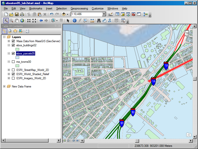
Once you have started ArcMap and loaded the datasets for this exercise, a zoom-in of the East Boston datasets in ArcMap will look something like this (with the building outlines shaded in light brown to help visualize the spatial structure). NOTE: you can get here faster by double clicking on this ArcMap document in your local copy of the datasets for this exercise: c:\temp\eboston05\eboston05_lab2start.mxd
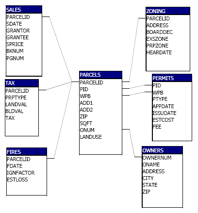
The attribute table for the East Boston parcel map (ebos_parcels05) layer has only a few geographic identifiers and none of the land use information from the assessing data. Before we can join the assessing data to the parcel map, however, we need to handle some of the one-to-many complications (due to condos). We will also want to match the East Boston land use codes to the categories and symbology recommended by the American Planning Association.
Preparing the Assessing Tables
Open your local copy of the East Boston MS-Access database, bos05eb_lab2.mdb. Note the descriptions of the various tables and queries already included in the database. Highlight the 'tables' object and double-click on bos05eb. This is the main table containing assessing information for East Boston land and properties. Highlight that table (by clicking once on the name) and then right-click on the table and choose the Design option in the menu to see the table schema and description of the attribute fields. (We have described the fields that will be useful for this lab.) We have also added some metadata to explain the tables. Right-click on a table and choose 'properties' to see the description of any particular table.
Creating a thematic map of East Boston land use is not hard - once we identify the appropriate information in the assessing tables and move it into ArcMap in a form that is ready for mapping. However, there are three difficulties that we have to overcome:
Difficulty #1: One-to-many issues in handling condos: Note that East Boston has 6,558 ground parcels (in the shapefile) but 7,235 records in the assessing table (for FY2005). A few of the parcel IDs in the assessing data will not match any of the parcels in the shapefile. However, the main reason for the different numbers is because condominiums generally have more than one separately owned housing or business unit located on a single 'ground' parcel.
In the case of Boston's assessing records, it gets even more complicated. The Boston assessing tables are not 'normalized' to insure that every record (that is every row) in the table has the same meaning as every other row for each attribute field (that is, column). In most cases, each row contains information about a single 'ground' parcel (and any property on the parcel). Every square foot of East Boston is contained in one or another of the non-overlapping ground parcels. The first column, PID, is usually the parcel ID for the ground parcel. However, in the case of condominiums, the condo units are taxed separately and generally have different property characteristics and different owners. To record all this information, the assessing table handles condos by including one row for each condo unit plus an additional row for the ground parcel (and the assessment information about the land and property held in common by the condo association). The row with ground parcel information contains the ground parcel ID for the condo in the PID column (just as for non-condo parcel records), but the rows describing individual condo units contain the condo unit ID in the PID column. This ID has the same first seven characters as the ground parcel ID and differs only in the last three digits (allowing for up to 1000 units in a condominium). You can tell which rows refer to condos by examining the second column, CM_ID (which stands for condominium-main ID). If the value in this column is null (that is, empty), then the row is not a condo, otherwise the value is the ground parcel ID for the condo. We will handle these condo complexities on the MS-Access database side and pull into ArcMap a simpler assessing table that is ready for mapping.
Difficulty #2: dBase format limitations: There is one more data definition complication that will hamper our efforts to link the assessing data to the parcel map. ArcGIS shapefiles use a dBase format for encoding tabular data (the data tables ending in *.dbf) and the dBase format can distinguish only the first 10 characters of field names. Actually, ArcMap uses a dBase format that *can* handle more than 10 characters in the name,but the ODBC (open data base connect) driver that we use to connect ArcMap to MS-Access uses internal tools that cannot handle dBase files with field names longer than 10 characters.
The East Boston assessing tables have three field names with the same first 10 characters. To overcome this difficulty, we have already shortened the three long field names to be: n_units_r, n_units_c, and n_units_rc instead of sec_num_units_r, etc. We will not even use these three fields in the exercise - but beware that we would have had trouble had we tried to copy the entire table into ArcMap. In fact, ArcMap would not complain about importing the table and it would look fine, but if we tried to join the table to the parcel table none of the rows would match properly!
Instead of trying to move the entire assessing table into ArcMap, we will construct a query to pull only the columns that we need. For large and complex table handling, this practice is often helpful - both for flexibility, ease of documentation, and to avoid problems such as the one just mentioned with importing data that we do not even need.
Difficulty #3: Data type mismatches: The East Boston assessing table uses the three-digit numeric state land use classification codes (called ptype in the table) that are required by the Mass Department of Revenue, DOR (http://www.mass.gov/dor/docs/dls/bla/classificationcodebook.pdf). We want to shade our land use map with the colors recommended by the APA land-based classification standards, LBCS (http://www.planning.org/lbcs). The APA standards are more complicated and distinguish land use instances that might apply to an activity, site, structure, function, or ownership category. To avoid making this lab exercise unduly long, we have already created a (simplistic) association between Mass DOR categories and the LBCS for land use activities. The 'lookup' table called MASS_LANDUSE in bos05eb_lab2.mdb lists all the DOR property type codes as well an approximate LBCS code.
The mass_landuse table also helps us with one other complexity. The East Boston assessing table encodes property type (ptype) as a 3-character alphanumeric field but the original DOR mass_landuse table encodes property type (stateclass) as a 3-digit integer. To address this difficulty, we have already run an 'update' query to populate the last column of mass_landuse (stclass_txt) with state class codes that have been converted to a 3-character text field. (The update query is also saved in bos05eb_lab2.mdb for your information but you do not need to rerun it.) Note that this issue is more than a simple data type conversion. Codes < 100 are expressed as two-digit numbers but, for example, the code = 22 should be sorted as '022' rather than '220' and you could have trouble matching codes if you are not careful about how to convert. This is a common problem when cross-referencing our '02139' zipcode.
Difficulty #4: Spaces buried in column names: The East Boston assessing table (bos05eb) is provided exactly as it was made available by the Assessing Office. The column labeled 'FY2005_ LAND' comes with a space ' ' in between the underscore and 'L'. Not only is it hard to see that there is a space in the name, but also the space is an invitation to future trouble. When you manipulate the table in MS-Access, you will see that the name is included within square brakcets [] so that MS-Access is not confused. But when you try to pull the table into ArcGIS or Postgres, the space will cause troubles if you do not take care to enclose the column name within quotes (either single quotes or double quotes depending upon the software package!). Be aware of this issue and, for example, rename the column on the fly to an acceptable name whenever you pull this column into a SQL query.
PREPARE A NEW MS-ACCESS QUERY that does the following:
- joins the assessing table to mass_landuse by matching ptype with stclass_txt
- has only one row per ground parcel for each East Boston parcel,
- handles condos by selecting only the condo-main (ground parcel) row and replaces the following square footage and tax fields with the sum from the other rows for that condo: gross_area, living_area, fy2005_total, fy2005_land, fy2005_bldg, gross_tax
- pulls the following columns from the two joined tables: PID, ST_NUM, ST_NAME, ST_NAME_SFX, PTYPE, LU, LOTSIZE, GROSS_AREA, LIVING_AREA, FY2005_TOTAL, FY2005_LAND, FY2005_BLDG, GROSS_TAX, NUM_FLOORS, LBCS, and stclass_txt
We suggest that you build this query in four stages. First prepare a query (q_noncondo) that pulls from the assessing table the desired columns for every row that refers to a non-condo ground parcel. In the case of condos, we only want the rows where LU=CM. (Ignore those few records where the CM_ID field is not null but the landuse is not CM. These are special cases that we do not consider in this lab!) Let's use this q_noncondo query to make a new table called t_noncondo. We choose the Query/Make-Table option and make a new table instead of just saving the q_noncondo as a query (without the 'make-table' option) since the 'append' command in the next step requires that you start with an actual table and add rows to it. Next, prepare a query (q_condosum) that pulls the desired columns from the assessing table for each of the condos and uses the SUM function to add up (in the correct columns) all of the square footage and tax amounts for each particular condominium association in order to include the totals in a single record for each condo association. Third, combine the first two queries (using the APPEND type of MS-Access query) to expand t_noncondo so that it has one row for each mapable parcel in East Boston (i.e., one row for each condo plus all the original rows for the non-condos). Finally, join this appended table with 'mass_landuse' to lookup the LBCS classification code. Call this final query q_eb05new.
To speed up the lab exercise, we have already created the 'group by' query (called 'q_condosum) and the 'append' query (called q_ebunion) that combines q_noncondo and q_condosum. Note, in order to use the q_ebunion query to append the q_condosum rows to the t_noncondo table that you created, you must have created t_noncondo with the same columns in the same order as the table returned by the q_condosum query.
What to turn in: Include in your lab assignment, the text of your queries q_noncondo and q_eb05new.
Mapping the Assessing Data
ArcMap sometimes has trouble with data types when importing data directly from MS-Access queries (without first creating the table in MS-Access). To avoid these issues, you may wish to modify your query q_eb05new so that it saves a table (call it eb05new) inside MS-Access.
Open the ArcMap document called eboston05_lab2.mxd that is saved inside your local copy of the eboston05 folder. Add the table, eb05new, that you just created in MS-Access. Join the eb05new table to the mapable ebos_parcels05 layer.
Next, we need the color shading scheme that we want to use for the various land uses. The Data Frame labeled 'LBCS Color Scheme' shows the various colors that the APA recommends for land use maps. We don't need to manipulate anything in this Data Frame - they are just there so you can see the land use category names and major colors. (If you are interested, take a look at the APA specs (http://www.planning.org/lbcs) describing the standard. You are supposed to pick an intensity of color to differentiate within a category. For example, residential is yellow. You can shade a darker color for housing that is more dense and lighter yellow for single family homes on large lots.) For now, we have already included an (approximate) LBCS land use code in our eb05new table and we will simply load the symbol description layer that APA provides for shading the main land use categories. Make sure the East Boston Parcels Data Frame is active and double-click on the ebos_parcels05 layer. Click on the 'symbology' tab and set the 'fields' value to 'eb05new.lbcs'. Next, click the 'Import' label and click the radio button that gets the layer definitions from an ArcView 3 legend file (*.avl). Navigate to the LBCS sub-folder and click on 'activity.avl'. Import the complete symbol definition and be sure to pick eb05new.lbcs as the field containing the land use code to be mapped. You may also want to set the properties for all symbols (click the 'symbol' label at the top of the legend) so that the parcel outlines are a light gray. The thematic map will now shade the parcels in a manner similar to that shown in the map above in this exercise.
In subsequent labs, we will return to these East Boston datasets and examine land value and population density in more detail. Think about what you would have to do at this point to shade the parcel map in a way that usefully represented land value and density.