This part of the exercise repeats the example provided last week but uses the newly installed 32-bit R and adds some additional options and steps. You can cut-and-paste the R commands into the R-Console window.
(1) Copy the data to a local driver: Use Windows Explorer to copy the entire MiniClass data locker (180 MB)
- From: Z:\course\11\11.523\data_ua
- To: C:\TEMP
(2) Use the RODBC package to open a data channel to MS-Access via the built-in ODBC 'machine data source' named 'MS Access Database'
- library("RODBC",lib.loc="c:\\temp\\rlib")
- UAchannel <- odbcConnect("MS Access Database",uid="")
- In the popup window, navigate to your copy of the miniclass data that you have copied from the class data locker
into c:\temp\rlib and select the MS-Access database: vmt_data.mdb - To close this connection exit from R or use the command: odbcClose(UAchannel)
- In the popup window, navigate to your copy of the miniclass data that you have copied from the class data locker
(3) Next, use this UAchannel to pull each of the four data tables from MS-Access into data frames in R
- demdata <- sqlFetch(UAchannel, "demographic_bg")
- bedata <- sqlFetch(UAchannel, "built_environment_250m")
- vmtdata <- sqlFetch(UAchannel, "vmt_250m")
- ctdata <- sqlFetch(UAchannel, "ct_grid")
(4) Use the matrix manipulation commands of R to check that the tables are properly read in and make sense
Command Result Comment
dim(demdata) [1] 3323 18 3323 rows and 18 columns dim(bedata)
[1] 117196 33 117196 rows and 22 columns dim(vmtdata) [1] 60895 21 117196 rows and 21 columns dim(ctdata) [1] 118668 6 118668 rows and 6 columns ctdata[1,]
1 1 19 34 Regional Cities
TOWN_NAME CODAs
1 Amesbury 1
xxx[1,] displays all the columns of row=1 from the array 'xxx' summary(ctdata)
Min. :1 Min. : 19 Min. : 34
1st Qu.:1 1st Qu.: 75668 1st Qu.: 75118
Median :1 Median :174345 Median :173760
Mean :1 Mean :166050 Mean :165844
3rd Qu.:1 3rd Qu.:261092 3rd Qu.:261147
Max. :2 Max. :314601 Max. :314374
Community_ TOWN_NAME
Developing Suburbs:65288 Plymouth : 4276
Inner Core : 6125 Middleborough: 3003
Maturing Suburbs :30513 Boston : 2099
Regional Cities :16742 Taunton : 1985
Carver : 1644
Ipswich : 1514
(Other) :104147
CODAs
Min. :0.0000
1st Qu.:0.0000
Median :0.0000
Mean :0.2595
3rd Qu.:1.0000
Max. :1.0000
(5) Get descriptive statistics for the demographic data table:
summary(demdata) ## note the missing values (NA's) for some of the variables BG_ID CT_ID PCT_sch13 Min. :2.501e+11 Min. :2.501e+10 Min. :0.2689 1st Qu.:2.502e+11 1st Qu.:2.502e+10 1st Qu.:0.8022 Median :2.502e+11 Median :2.502e+10 Median :0.8922 Mean :2.502e+11 Mean :2.502e+10 Mean :0.8543 3rd Qu.:2.502e+11 3rd Qu.:2.502e+10 3rd Qu.:0.9431 Max. :2.503e+11 Max. :2.503e+10 Max. :1.0000 NA's :6 PCT_owner INC_MED_HS PCT_pov PCT_white Min. :0.0000 Min. : 0 Min. :0.00000 Min. :0.0000 1st Qu.:0.3869 1st Qu.: 41544 1st Qu.:0.02464 1st Qu.:0.7586 Median :0.6458 Median : 55284 Median :0.05382 Median :0.9027 Mean :0.6125 Mean : 59057 Mean :0.09154 Mean :0.8171 3rd Qu.:0.8759 3rd Qu.: 71745 3rd Qu.:0.11828 3rd Qu.:0.9633 Max. :1.0000 Max. :200001 Max. :0.84164 Max. :1.1642 NA's :8 NA's :6 NA's :4 PCT_under5 PCT_old65 pct_ov2car INC_CAPITA Min. :0.00000 Min. :0.00000 Min. :0.00000 Min. : 0 1st Qu.:0.05283 1st Qu.:0.07864 1st Qu.:0.05466 1st Qu.: 20045 Median :0.07476 Median :0.11993 Median :0.11227 Median : 25548 Mean :0.07528 Mean :0.13000 Mean :0.12512 Mean : 28052 3rd Qu.:0.09645 3rd Qu.:0.16688 3rd Qu.:0.18182 3rd Qu.: 32804 Max. :0.32477 Max. :0.62932 Max. :0.52863 Max. :122938 NA's :4 NA's :4 NA's :8 pct_elsc_sch pct_less3hsh pct_labor pct_unempl Min. :0.0000 Min. :0.1385 Min. :0.0000 Min. :0.00000 1st Qu.:0.1329 1st Qu.:0.4688 1st Qu.:0.6194 1st Qu.:0.01570 Median :0.1821 Median :0.5632 Median :0.6844 Median :0.03187 Mean :0.1803 Mean :0.5718 Mean :0.6705 Mean :0.04446 3rd Qu.:0.2277 3rd Qu.:0.6610 3rd Qu.:0.7370 3rd Qu.:0.05609 Max. :0.6148 Max. :1.0000 Max. :1.0000 Max. :0.76060 NA's :4 NA's :8 NA's :4 NA's :6 F1_wealth F2_children F3_working Min. :-4.0844 Min. :-3.48684 Min. :-6.90175 1st Qu.:-0.4908 1st Qu.:-0.59101 1st Qu.:-0.50150 Median : 0.2355 Median : 0.06503 Median : 0.08234 Mean : 0.0000 Mean : 0.00000 Mean : 0.00000 3rd Qu.: 0.6952 3rd Qu.: 0.72343 3rd Qu.: 0.61345 Max. : 2.6100 Max. : 3.43180 Max. : 3.92767 NA's :9 NA's :9 NA's :9
(6) Exclude certain rows and columns so that the factor analysis works and is more meaningful
For a nice discussion of Factor analysis see: http://en.wikipedia.org/wiki/Factor_analysis For a more extensive discussion of factor analysis, principal component analysis, and the interpretation of results, take a look at Chapter 6 of Sumeeta Srinivasan's PhD dissertation (DUSP/UIS PhD, 2000), "Linking land use and transportation: measuring the impact of neighborhood-scale spatial patterns on travel behavior," Massachusetts Institute of Technology: Urban Studies and Planning, PhD Dissertation: http://mit.dspace.org/handle/1721.1/70335?show=full
We should exclude the first and last few columns from the data frame before doing a factor analysis. (The first two are the block group and census tract IDs and the last three are the first three demographic factors computed in Mi Diao's thesis.
Create list of columns to remove from consideration and apply it to demdata to create demdata2
- outlist <- c("BG_ID","CT_ID","F1_wealth","F2_children","F3_working")
- demdata2 <- demdata[,setdiff(names(demdata),outlist)]
Double check the dimensions and a few rows of the result in demdata2 and try a factor analysis (using varimax by default for the rotation of the factors)
- fac3 <- factanal(demdata2, factors=3)
Error in cov.wt(z) : 'x' must contain finite values onlyOops, there are still problems with missing values in the data. Let's only consider block groups where household income >0.
- demdata3 <- demdata2[demdata2[,'INC_MED_HS']>0,]
- dim(demdata3)
[1] 3315 13- fac3 <- factanal(demdata2, factors=3)
Error in cov.wt(z) : 'x' must contain finite values onlyHmm, the right number of rows and columns, but still some problems. Let's use the 'complete.cases' command to retain only those rows that are complete cases:
- demdata4 <- demdata2[complete.cases(demdata2),]
dim(demdata4)
[1] 3314 13- << Note: building demdata4 from demdata3 instead of demdata2 will yield the same result since all the complete cases happen to have INC_MED_HS > 0 >>
Okay, one more row is eliminated and now the factor analysis works:
- fac4 <- factanal(demdata4, factors=3)
- fac4
Call:
         factanal(x = demdata4, factors = 3)
Uniquenesses: PCT_sch13 PCT_owner INC_MED_HS PCT_pov PCT_white 0.246 0.183 0.321 0.289 0.384 PCT_under5 PCT_old65 pct_ov2car INC_CAPITA pct_elsc_sch 0.688 0.005 0.389 0.518 0.375 pct_less3hsh pct_labor pct_unempl 0.083 0.412 0.725Loadings: Factor1 Factor2 Factor3 PCT_sch13 0.815 -0.202 0.220 PCT_owner 0.818 0.380 INC_MED_HS 0.778 0.217 0.163 PCT_pov -0.842 PCT_white 0.764 -0.170 PCT_under5 0.552 PCT_old65 0.205 -0.324 -0.921 pct_ov2car 0.623 0.470 INC_CAPITA 0.649 -0.216 0.116 pct_elsc_sch -0.145 0.775 pct_less3hsh -0.109 -0.946 pct_labor 0.452 0.619 pct_unempl -0.518Factor1 Factor2 Factor3 SS loadings 4.593 2.438 1.351 Proportion Var 0.353 0.188 0.104 Cumulative Var 0.353 0.541 0.645Test of the hypothesis that 3 factors are sufficient. The chi square statistic is 4112.4 on 42 degrees of freedom. The p-value is 0This output is okay and looks similar to Mi Diao's results but has one extra variable (pct_ov2car). Create a list with that column heading and use it to toss that column
- outlist <- c("pct_ov2car")
- demdata5 <-demdata4[,setdiff(names(demdata4),outlist)]
- dim(demdata5)
[1] 3314 12Okay, that column is eliminated, now try the factor analysis again
- fac5 <- factanal(demdata5, factors=3) # varimax is the default
- fac5
Call:
         factanal(x = demdata5, factors = 3)
Uniquenesses: PCT_sch13 PCT_owner INC_MED_HS PCT_pov PCT_white PCT_under5 0.241 0.193 0.315 0.284 0.395 0.679 PCT_old65 INC_CAPITA pct_elsc_sch pct_less3hsh pct_labor pct_unempl 0.005 0.510 0.363 0.095 0.410 0.724Loadings: Factor1 Factor2 Factor3 PCT_sch13 0.819 -0.198 0.219 PCT_owner 0.811 0.382 INC_MED_HS 0.781 0.221 0.163 PCT_pov -0.846 PCT_white 0.756 -0.171 PCT_under5 0.560 PCT_old65 0.206 -0.323 -0.921 INC_CAPITA 0.659 -0.207 0.115 pct_elsc_sch -0.144 0.783 pct_less3hsh -0.105 -0.940 -0.102 pct_labor 0.454 0.620 pct_unempl -0.519Factor1 Factor2 Factor3 SS loadings 4.210 2.225 1.350 Proportion Var 0.351 0.185 0.113 Cumulative Var 0.351 0.536 0.649Test of the hypothesis that 3 factors are sufficient. The chi square statistic is 3792.42 on 33 degrees of freedom. The p-value is 0This works and is similar to Prof. Diao's (except that factors lower than 0.35 are not omitted). We can get even closer to Prof. Diao's results by using a slightly different procedure: principal components analysis (PCA).
- prin5 <- principal(demdata5, nfactors=3, rotate="varimax")
prin5 # print results
Principal Components Analysis
         Call: principal(r = demdata5, nfactors = 3, rotate = "varimax")
         Standardized loadings (pattern matrix) based upon correlation matrix
                PC1   PC2   PC3   h2   u2
 PCT_sch13     0.82 -0.20  0.27 0.78 0.22
 PCT_owner     0.82  0.39 -0.05 0.82 0.18
 INC_MED_HS    0.81  0.22  0.19 0.75 0.25
 PCT_pov      -0.86 -0.03 -0.04 0.75 0.25
 PCT_white     0.80 -0.18 -0.07 0.67 0.33
 PCT_under5   -0.02  0.73  0.06 0.53 0.47
 PCT_old65     0.23 -0.32 -0.86 0.89 0.11
 INC_CAPITA    0.71 -0.19  0.15 0.56 0.44
 pct_elsc_sch -0.14  0.87  0.04 0.78 0.22
 pct_less3hsh -0.10 -0.91 -0.13 0.85 0.15
 pct_labor     0.43 -0.05  0.79 0.81 0.19
 pct_unempl   -0.61  0.04  0.13 0.39 0.61
PC1 PC2 PC3 SS loadings 4.52 2.53 1.54 Proportion Var 0.38 0.21 0.13 Cumulative Var 0.38 0.59 0.72 Proportion Explained 0.53 0.29 0.18 Cumulative Proportion 0.53 0.82 1.00Test of the hypothesis that 3 components are sufficient.The degrees of freedom for the null model are 66 and the objective function was 8.01 The degrees of freedom for the model are 33 and the objective function was 1.61 The number of observations was 3314 with Chi Square = 5308.97 with prob < 0Fit based upon off diagonal values = 0.97These results match those of Prof Diao quite closely in Table 3 on page 45 (but our results include factors with low weights < 0.35). Try similar factor and principal component analysis for the other data table with built environment measures.
(7) GRAPHICS: Visualize data patterns using scattergrams and box plots.
Here is a useful reference regarding scatterplots in R: http://www.statmethods.net/graphs/scatterplot.html
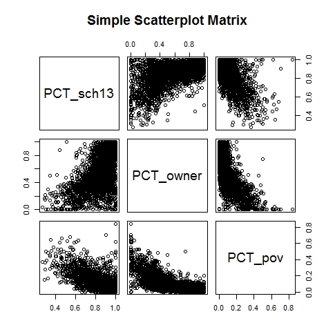
Let's plot scattergrams for pairs of the variables: pct_sch13, pct_owner, and pct_pov
- pairs(~PCT_sch13+PCT_owner+PCT_pov,data=demdata5,main="Simple Scatterplot Matrix")
Hmm, some of these relationships look somewhat non-linear - an issue since factor analysis is searching for linear combinations of variables that identify clusters of block groups with similar characteristics. We may want to transform some of the variables before doing the factor analysis. But, first, there are so many data points that it is hard to see what is happening in the point clouds.Let's use the 'hexbin' procedure to 'bin' the data into 50 groups along each dimension before we generate the scatterplots. That way, we can use different symbols on the graph depending on whether a 'bin' has a few or very many cases that fall within it.
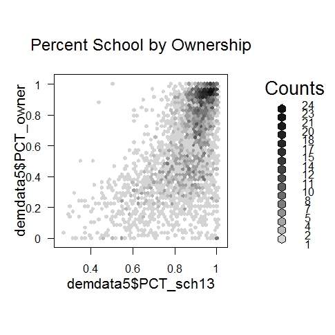
- bin <- hexbin(demdata5$PCT_sch13,demdata5$PCT_owner,xbins=50)
- plot(bin,main="Percent School by Ownership")
We see that homeownership and schooling are high together - a very common case in the upper right. Where homeownership is not so high (80+%), the relationship is much weaker between the home ownership percentage of a block group and the percent with some 13+ years of education.
Try examining other paris of variables to get a feel for the data and to being thinking about outliers and sub-markets where the relationships and relevant factors might be quite different. We will get back to some of these considerations in Part 3 when we consider alternative models and explore the possibility that the VMT/built-environment relationship may be different for different community types.
(8) Modeling VMT as a function of BE and Demographics
Next, lets fit the ordinary least squares (OLS) model in Prof. Diao's dissertation (Tables 5 and 6) that models the average annual mileage per vehicle (VMT) for vehicles registered within a 250x250m grid cell as a function of the 5 built environment (BE) factors and the 3 demographic factors.
In order to fit the models, we need to join the three tables in demdata, bedata, and vmtdata so each row (for a unique grid cell) has that grid cells mileage estimate plus the 5 BE factors and 3 demographic factors. While we are doing this join, we might as well include one additional column - the community type associated with each grid cell. Recall that, in last Thursday's spatial data management session, we used the TAZ_attr shapefile that had the 'community type' designation by the Metropolitan Area Planning Council (MAPC) for every traffic analysis zone. (Actually, the type is designated for each of the 164 municipalities in the metro Boston region.) In our miniclass, we showed how to do a 'spatial join' in ArcGIS to tag each grid cell with the type of community that it was in. The results have been saved into a table called ct_grid in our vmt_data.mdb database. We have already read this table into an R data frame called, ctdata.
We could use R tools to merge the four tables, but complex relational joins in R can be combersome and condusive to errors. Instead, let's join the four tables in MS-Access, bring over to R only the 10 columns of data (plus grid cell and block group IDs) for each grid cell, and doing our modeling with that table. Actually, we will want to bring over a few more columns indicating the number of households estimated to be in each grid cell, the quality of VMT estimate, and the like. (See page 44 of the dissertation regarding which grid cells are included in the modeling.)
For your convenience, we have already built and saved the query in MS-Access that joins the 4 tables to produce a new table, t_vmt_join4, with 60377 rows. (Note that, to be a row in this table, a grid cell had to have estimates of VMT and all 8 factors.) Pull this table into a new data frame in R and use 'complete.cases' to omit rows with missing values:
- vmt_join <- sqlFetch(UAchannel, "t_vmt_join4")
- dim(vmt_join)
[1] 53429 19- vmtall <- vmt_join[complete.cases(vmt_join),]
- dim(vmtall)
[1] 53250 19- vmtall[1,]
  g250m        bg_id  vmt_vin  f1_nw f2_connect f3_transit  f4_auto
1    65 250092671024 13270.79 0.4439   -0.16947    1.10299 -0.13811
   f5_walk f1_wealth  f2_kids  f3_work                 ct hshld_2000
1 -0.55755 0.8841909 1.669427 1.004693 Developing Suburbs      8.727
  vmt_pop vmt_hh no_vin no_good vmt_tot_mv vin_mv
1   20971  59306     39      33    1186400    105
Note that my MS-Access query to join the tables also changed the names of a few columns to make them lower case and shorter. Now we are ready to run a simple ordinary least squares regression of VMT per vin on the 8 BE and 3 Demographic factors:
- run_ols1 <- lm(formula = vmt_vin ~ f1_nw + f2_connect + f3_transit + f4_auto + f5_walk +f1_wealth +f2_kids + f3_work, data=vmtall)
- summary(run_ols1)
Call: Call: lm(formula = (vmt_tot_mv/vin_mv) ~ f1_nw + f2_connect + f3_transit + f4_auto + f5_walk + f1_wealth + f2_kids + f3_work, data = vmtall) Residuals: Min 1Q Median 3Q Max -11701.6 -727.7 -34.7 704.2 10887.1 Coefficients: Estimate Std. Error t value Pr(>|t|) (Intercept) 12596.789 10.807 1165.63 <2e-16 *** f1_nw 698.115 7.080 98.60 <2e-16 *** f2_connect -472.713 5.815 -81.29 <2e-16 *** f3_transit 858.899 5.890 145.82 <2e-16 *** f4_auto 164.073 8.735 18.78 <2e-16 *** f5_walk -146.136 6.284 -23.26 <2e-16 *** f1_wealth -246.211 10.714 -22.98 <2e-16 *** f2_kids 201.393 8.571 23.50 <2e-16 *** f3_work 198.404 6.849 28.97 <2e-16 *** --- Signif. codes: 0 *** 0.001 ** 0.01 * 0.05 . 0.1 1 Residual standard error: 1244 on 53241 degrees of freedom Multiple R-squared: 0.5183, Adjusted R-squared: 0.5182 F-statistic: 7160 on 8 and 53241 DF, p-value: < 2.2e-16Hmm, the model coefficients have similar signs and values but much lower R-squared than reported in the dissertation. That is because vmt_vin is the estimated mileage for individual grid cells and there are many grid cells with few vehicles and noisy estimates. Instead of using individual grid cells, Prof Diao average the numbers in the 9-cell window around each grid cell. We can do this by dividing vmt_tot_mv by vmt_mv in the vmt_250m table. The vmt_tot_mv column is the total mileage for the 9-cell window and vmt_mv is the total number of vehicles in the 9-cell region. So let's regress vmt_tot_mv / vmt_mv on the left hand side (taking care to do the division only for grid cells that had vmt_mv > 0.
- run_ols1 <- lm(formula = (vmt_tot_mv / vin_mv) ~ f1_nw + f2_connect + f3_transit + f4_auto + f5_walk +f1_wealth +f2_kids + f3_work, data=vmtall)
- summary(run_ols1)
Call:
         lm(formula = (vmt_tot_mv/vin_mv) ~ f1_nw + f2_connect + f3_transit +
 f4_auto + f5_walk + f1_wealth + f2_kids + f3_work, data = vmt_join)
Residuals: Min 1Q Median 3Q Max -11701.7 -727.9 -35.4 704.4 10883.1Coefficients: Estimate Std. Error t value Pr(>|t|) (Intercept) 12596.906 10.786 1167.88 <2e-16 *** f1_nw 698.492 7.071 98.78 <2e-16 *** f2_connect -472.531 5.815 -81.26 <2e-16 *** f3_transit 859.571 5.885 146.07 <2e-16 *** f4_auto 165.860 8.723 19.01 <2e-16 *** f5_walk -145.796 6.284 -23.20 <2e-16 *** f1_wealth -245.697 10.701 -22.96 <2e-16 *** f2_kids 201.831 8.572 23.55 <2e-16 *** f3_work 196.183 6.841 28.68 <2e-16 *** --- Signif. codes: 0 ‘***’ 0.001 ‘**’ 0.01 ‘*’ 0.05 ‘.’ 0.1 ‘ ’ 1Residual standard error: 1246 on 53412 degrees of freedom (8 observations deleted due to missingness) Multiple R-squared: 0.5177, Adjusted R-squared: 0.5177 F-statistic: 7167 on 8 and 53412 DF, p-value: < 2.2e-16Okay, this looks much better, and gives an indication of how much noise there is in the individual grid cells - at least in the suburbs where the density is much lower. We still have only produced the ordinary least squares results and have not adjusted for spatial autocorrelation (so the coefficients are not directly comparable to any of the results shown in the dissertation).
(9) Good references for further work with R
- An online 'Quick-R' reference: www.statmethods.net
- A paperbook (or e-book) that I find to be a useful reference for data manipulation and basic stats
oreilly.com
R in a Nutshell: A Desktop Quick Reference
Joseph Adler, O'Reilly
2nd edition, 2012 (Sept.)paperbook $49.99 at O'Reilly:
http://shop.oreilly.com/product/0636920022008.do
($35.99 as Ebook)paperbook $37.05 at Amazon
http://www.amazon.com/R-Nutshell-OReilly-Joseph-Adler/dp/144931208X/ref=sr_1_2?s=books&ie=UTF8&qid=1350371375&sr=1-2&keywords=r+in+a+nutshellkindle version: $19.79