Thin Shear Layer Approximation
Thin Shear Layer Approximation
1 Viscous flow equations
Steady incompressible laminar viscous flow is described by
the Navier-Stokes Equations together with
appropriate boundary conditions.
Near a solid wall, the tangential velocity goes to its zero
no-slip value through a thin thear layer of thickness d,
which varies depending on the distance L to the leading edge
as shown in Figure . At large Reynolds numbers
ue L/n >> 1, the shear layer becomes very slender such that
d/L << 1.
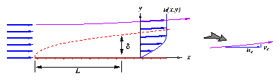
Figure 1: Thin shear layer geometry and velocities.
2 Scales and ordering
For a slender shear layer, scales for the velocities
and velocity gradients can be obtained from
the edge velocity values ue, ve.
The last pressure gradient scale follows from the Bernoulli relation
which is valid outside the shear layer.
Ordering the terms in the continuity equation
and the self-evident requirement that the only two terms
in the equation must be of the same order,
produces the scaling rule for the vertical velocity v.
The terms in the x-momentum equation have the following ordering.
Since d << L, the first viscous term can be clearly neglected
over the second. The remaining terms then produce an order estimate
for the shear layer fineness ratio d/L.
|
| |
|
|
| |
|
|
O |
Õ
õ
Š
|
|
Ì
Ó
Ò
|
|
n
ue L
|
|
—
¼
½
|
1/2
|
|
ª
º
«
|
= O |
Ì
Ó
Ò
|
|
1
ReL1/2
|
|
—
¼
½
|
|
|
| |
|
Ordering the terms in the y-momentum equation
produces the conclusion that the normal pressure gradient is
or higher order than the streamwise pressure gradient.
|
| |
|
|
|
O |
Ì
Ó
Ò
|
|
d
L
|
|
ue2
L
|
|
—
¼
½
|
= O |
Ì
Ó
Ò
|
|
d
L
|
|
1
r
|
|
Ñp
Ñx
|
|
—
¼
½
|
|
|
| |
|
The difference in pressure Dpy across the shear layer is
clearly negligible to the differences in pressure Dpx
along the shear layer.
|
|
|
Dpy ~ d |
Ñp
Ñy
|
= O |
Ì
Ó
Ò
|
ue2 |
d2
L2
|
|
—
¼
½
|
|
|
|
|
| |
|
For a curved wall, the leading-order approximation to the
normal pressure gradient becomes
where k is the wall curvature.
In this case,
|
|
|
Dpy ~ d |
Ñp
Ñy
|
= O ( ue2 kd) |
|
|
|
| |
|
and the pressure differences across the shear layer are still small,
since kd << 1 is typical of most shear layer situations.
This analysis indicates that the pressure can be assumed constant
across the shear layer.
The pressure gradient term can then be expressed only in terms of
the tangential edge velocity.
|
| |
| |
- |
1
r
|
|
Ñp
Ñx
|
@ - |
1
r
|
|
d pe
d x
|
= ue |
d ue
d x
|
|
|
| |
|
3 Thin Shear Layer Equations
The above analysis shows that for large Reynolds numbers,
the steady incompressible Navier-Stokes equations can be reduced
to the simpler Thin Shear Layer Equations.
The derivation was based on considering of the flat-plate geometry
in Figure 1, although these equations are also valid
for boundary layers on curved walls and free shear layers and wakes
along curved streamlines, provided the
In such cases the coordinate x is the
arc length along the layer, y is the transverse distance, and u,v
are the respective streamwise and transverse velocity components
as shown in Figure .
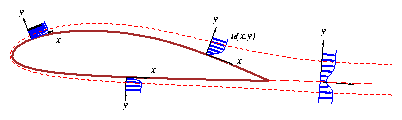
Figure 2: Curved shear layers and coordinates.
4 Thin Shear Layer Categories
Equations (2) are valid for all types of shear layers,
which are distinguished by different initial and boundary conditions.
The general initial condition at xo is
The various possible downstream boundary conditions
for x > xo are given below.
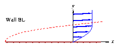
4.1 Wall boundary layer
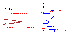
For a symmetric wake, suitable boundary conditions are:
|
| |
|
| |
|
Ñu/Ñy(x,0) = 0, v(x,0) = 0 |
|
| |
|
while for a general assymetric wake they are:
The ``centerline'' position yc and specified vertical velocity vc
are both arbitrary, provided vc << ue.
This condition merely serves to position the x,y
coordinate system within the shear layer flowfield.
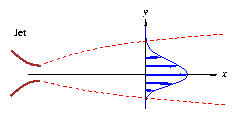
4.3 Mixing layer
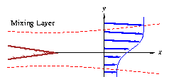
This differs from the wake in that the top and bottom potential
flows have different velocities and hence different total pressure.