17.1 The Reynolds Analogy
We describe the physical
mechanism for the heat transfer coefficient in a turbulent
boundary layer because most aerospace vehicle applications have
turbulent boundary layers. The treatment closely follows that in
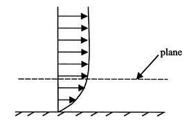
Eckert and Drake (1959). Very near the wall, the fluid motion is
smooth and laminar, and molecular conduction and shear are
important. The shear stress,  , at a plane is given by
 (where
  is the dynamic viscosity), and the
heat flux by
is the dynamic viscosity), and the
heat flux by
 . The latter is the same
expression that was used for a solid. The boundary layer is a region
in which the velocity is lower than the free stream as shown in
Figures 17.2 and
17.3. In a turbulent boundary
layer, the dominant mechanisms of shear stress and heat transfer
change in nature as one moves away from the wall.
. The latter is the same
expression that was used for a solid. The boundary layer is a region
in which the velocity is lower than the free stream as shown in
Figures 17.2 and
17.3. In a turbulent boundary
layer, the dominant mechanisms of shear stress and heat transfer
change in nature as one moves away from the wall.
Figure 17.3:
Velocity profile
near a surface
|
|
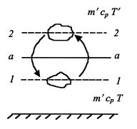
As one moves away from the wall (but still in the boundary layer),
the flow is turbulent. The fluid particles move in random directions
and the transfer of momentum and energy is mainly through
interchange of fluid particles, shown schematically in
Figure 17.4.
Figure 17.4:
Momentum and
energy exchanges in turbulent flow
|
|
With reference to Figure 17.4,
because of the turbulent velocity field, a fluid mass  penetrates the plane
  per unit time and unit area. In steady
flow, the same amount crosses
from the other side. Fluid moving
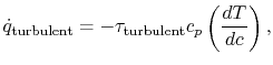
up transports heat
per unit time and unit area. In steady
flow, the same amount crosses
from the other side. Fluid moving
up transports heat  . Fluid moving down transports
  downwards. If
  , there is a turbulent downwards heat flow
 , given by
 , that results.
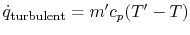
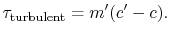
Fluid moving up also has momentum  and fluid moving down has
momentum
and fluid moving down has
momentum  . The net flux of momentum down per unit area and
time is therefore
. The net flux of momentum down per unit area and
time is therefore  . This net flux of momentum per unit
area and time is a force per unit area or stress, given by
. This net flux of momentum per unit
area and time is a force per unit area or stress, given by
 |
(17..3) |
Based on these considerations, the relation between heat flux and
shear stress at plane
is
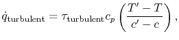 |
(17..4) |
or (again approximately)
 |
(17..5) |
since the locations of planes 1-1 and 2-2 are arbitrary.
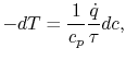
For the laminar region, the heat flux towards the wall is
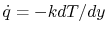 and dividing by the expression for the shear stress,
 , yields
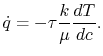 |
(17..6) |
The same relationship is applicable in laminar or turbulent flow if
 or, expressed slightly differently,
 |
(17..7) |
where  is the kinematic viscosity, and
  is the thermal
diffusivity.
is the thermal
diffusivity.
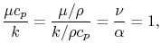
The quantity  is known as the Prandtl number (
 ),
after the man who first presented the idea of the boundary layer and
was one of the pioneers of modern fluid mechanics. For gases,
Prandtl numbers are in fact close to unity and for air
),
after the man who first presented the idea of the boundary layer and
was one of the pioneers of modern fluid mechanics. For gases,
Prandtl numbers are in fact close to unity and for air  at room temperature. The Prandtl number varies little over a wide
range of temperatures: approximately 3% from 300-2000
K.
at room temperature. The Prandtl number varies little over a wide
range of temperatures: approximately 3% from 300-2000
K.
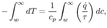
We want a relation between the values at the wall (at which  and
and  ) and those in the free stream. To get this, we
integrate the expression for
) and those in the free stream. To get this, we
integrate the expression for  from the wall to the free stream
 |
(17..8) |
where the relation between heat transfer and shear stress has been
taken as the same for both the laminar and the turbulent portions of
the boundary layer. The assumption being made is that the mechanisms
of heat and momentum transfer are similar.
Equation (17.8) can be integrated from the wall
to the freestream (conditions ``at  ''):
''):
 |
(17..9) |
where
 and
and  are assumed constant.
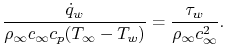
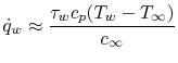
Carrying out the integration yields
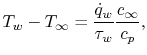 |
(17..10) |
where  is the velocity and
is the specific heat. In
Equation (17.10),
is the velocity and
is the specific heat. In
Equation (17.10),  is the
heat flux to the wall and
is the
heat flux to the wall and  is the shear stress at the wall.
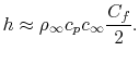
The relation between skin friction (shear stress) at the wall and
heat transfer is thus
is the shear stress at the wall.
The relation between skin friction (shear stress) at the wall and
heat transfer is thus
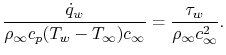 |
(17..11) |
The quantity
is known as the skin friction coefficient and is denoted by
 . The skin friction
coefficient has been tabulated (or computed) for a large number of
situations. If we define a non-dimensional quantity
. The skin friction
coefficient has been tabulated (or computed) for a large number of
situations. If we define a non-dimensional quantity
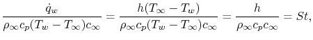 |
(17..12) |
known as the Stanton Number, we can write an expression for the heat
transfer coefficient,  as
as
 |
(17..13) |
Equation (17.13) provides a
useful estimate of
, or
, based on knowing the skin
friction, or drag. The direct relationship between the Stanton
Number and the skin friction coefficient is
 |
(17..14) |
The relation between the heat transfer and the skin friction
coefficient
 |
(17..15) |
is known as the Reynolds analogy between shear stress and
heat transfer. The Reynolds analogy is extremely useful in obtaining
a first approximation for heat transfer in situations in which the
shear stress is ``known.''
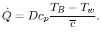
An example of the use of the Reynolds analogy is in analysis of a
heat exchanger. One type of heat exchanger has an array of tubes
with one fluid flowing inside and another fluid flowing outside,
with the objective of transferring heat between them. To begin, we
need to examine the flow resistance of a tube. For fully developed
flow in a tube, it is more appropriate to use an average velocity
 and a bulk temperature
  . Thus, an approximate
relation for the heat transfer is
. Thus, an approximate
relation for the heat transfer is
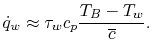 |
(17..16) |
The fluid resistance (drag) is all due to shear forces and is given
by
 , where
  is the tube ``wetted'' area
(perimeter
is the tube ``wetted'' area
(perimeter  length). The total heat transfer,
  , is
, is
 , so that
 |
(17..17) |
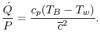
The power,  , to drive the flow through a resistance is given by
the product of the drag and the velocity,
, to drive the flow through a resistance is given by
the product of the drag and the velocity,
 , so that
 |
(17..18) |
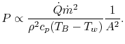
The mass flow rate is given by
 ,
where
,
where  is the cross sectional area. For a given mass flow rate
and overall heat transfer rate, the power scales as
is the cross sectional area. For a given mass flow rate
and overall heat transfer rate, the power scales as
 or as
or as  , i.e.,
 |
(17..19) |
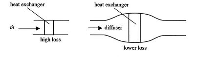
Equations (17.18) and
(17.19) show that to decrease the power
dissipated, we need to decrease
, which can be
accomplished by increasing the cross-sectional area. Two possible
heat exchanger configurations are sketched in
Figure 17.5; the one on the right will
have a lower loss.
Figure 17.5:
Heat exchanger configurations
|
|
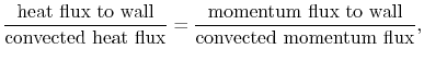
To recap, there is an approximate relation between skin
friction (momentum flux to the wall) and heat transfer called the
Reynolds analogy that provides a useful way to estimate heat
transfer rates in situations in which the skin friction is known.
The relation is expressed by
or
or
The Reynolds analogy can be used to give information about scaling
of various effects as well as initial estimates for heat transfer.
It is emphasized that it is a useful tool based on a hypothesis
about the mechanism of heat transfer and shear stress and not
a physical law.
Muddy Points
What is the ``analogy'' that we are discussing? Is it that the
equations are similar? (MP 17.2)
In what situations does the Reynolds analogy ``not work?''
(MP 17.3)
UnifiedTP
|