17.3 Dimensionless Numbers and Analysis of Results
Phenomena in fluid flow and heat transfer depend on
dimensionless parameters. The Mach number and the Reynolds
number are two you have already seen. These parameters give
information as to the relevant flow regimes of a given solution.
Casting equations in dimensionless form helps show the generality of
application to a broad class of situations (rather than just one set
of dimensional parameters). It is generally good practice to use
non-dimensional numbers, forms of equations, and results
presentation whenever possible. The results for heat transfer from
the cylinder are already in dimensionless form but we can carry the
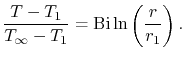
idea even further. For the cylinder, we had in
Equation (17.25),
The parameter  or
or  , where
  is a relevant length for
the particular problem of interest, is called the Biot
number, denoted by
is a relevant length for
the particular problem of interest, is called the Biot
number, denoted by
 . In terms of this parameter,
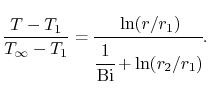 |
(17..29) |
The size of the Biot number gives a key to the regimes in which
different features are dominant. For
 the
convection heat transfer process offers little resistance to heat
transfer. There is thus only a small
the
convection heat transfer process offers little resistance to heat
transfer. There is thus only a small  outside (i.e.
 close to
  ) compared to the
through the
solid with a limiting behavior of
) compared to the
through the
solid with a limiting behavior of
as
goes to infinity. This is much like the situation
with an external temperature specified.
For
 the conduction heat transfer process offers
little resistance to heat transfer. The temperature difference in
the body (i.e. from
the conduction heat transfer process offers
little resistance to heat transfer. The temperature difference in
the body (i.e. from  to
to  ) is small compared to the
external temperature difference,
) is small compared to the
external temperature difference,
 . In this
situation, the limiting case is
. In this
situation, the limiting case is
In this regime there is approximately uniform temperature in the
cylinder. The size of the Biot number thus indicates the regimes
where the different effects become important.
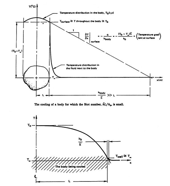
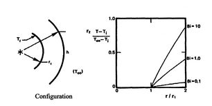
Figure 17.9 shows the general effect of Biot number
on temperature distribution. Figure 17.10 is a
plot of the temperature distribution in the cylinder for values of
 ,
,  and
and  .
.
Figure 17.9:
Effect of the Biot Number
 on the temperature distributions in the solid
and in the fluid for convective cooling of a body. Note that
on the temperature distributions in the solid
and in the fluid for convective cooling of a body. Note that
 is the thermal conductivity of the body,
not of the fluid. [from: A Heat Transfer Textbook,
John H. Lienhard, Prentice-Hall Publishers, 1980]
is the thermal conductivity of the body,
not of the fluid. [from: A Heat Transfer Textbook,
John H. Lienhard, Prentice-Hall Publishers, 1980]
|
|
Figure 17.10:
Temperature distribution in a
convectively cooled cylinder for different values of Biot number,
;  [from: A Heat Transfer Textbook,
John H. Lienhard, Prentice-Hall Publishers, 1980]
[from: A Heat Transfer Textbook,
John H. Lienhard, Prentice-Hall Publishers, 1980]
|
|
UnifiedTP
|