- Lost work in Adiabatic Throttling: Entropy and Stagnation Pressure Changes
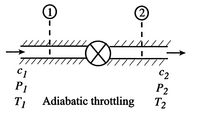
Figure 6.8:
Adiabatic Throttling
|
|
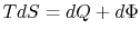
A process we have encountered before is adiabatic throttling of a
gas, by a valve or other device as shown in
Figure 6.8. The velocity is denoted by
 . There is no shaft work and no heat transfer and the flow is
steady. Under these conditions we can use the first law for a
control volume (the Steady Flow Energy Equation) to make a statement
about the conditions upstream and downstream of the valve:
. There is no shaft work and no heat transfer and the flow is
steady. Under these conditions we can use the first law for a
control volume (the Steady Flow Energy Equation) to make a statement
about the conditions upstream and downstream of the valve:
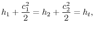
where  is the stagnation enthalpy, corresponding to a (possibly
fictitious) state with zero velocity. The stagnation enthalpy is the
same at stations 1 and 2 if
is the stagnation enthalpy, corresponding to a (possibly
fictitious) state with zero velocity. The stagnation enthalpy is the
same at stations 1 and 2 if  , even if the flow processes are
not reversible.
, even if the flow processes are
not reversible.
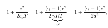
For a perfect gas with constant specific heats,  and
and
 . The relation between the static and stagnation
temperatures is:
. The relation between the static and stagnation
temperatures is:
where  is the speed of sound and
  is the Mach number,
  . In deriving this result, use has only been made of the first
law, the equation of state, the speed of sound, and the definition
of the Mach number. Nothing has yet been specified about whether the
process of stagnating the fluid is reversible or irreversible.
. In deriving this result, use has only been made of the first
law, the equation of state, the speed of sound, and the definition
of the Mach number. Nothing has yet been specified about whether the
process of stagnating the fluid is reversible or irreversible.
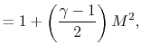
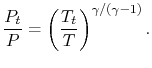
When we define the stagnation pressure, however, we do it with
respect to isentropic deceleration to the zero velocity state. For
an isentropic process
The relation between static and stagnation pressures is
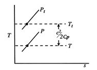
Figure 6.9:
Static and stagnation
pressures and temperatures
|
|
The stagnation state is defined by  ,
,  . In addition,
 . The static
and stagnation states are shown in
. The static
and stagnation states are shown in  -
- coordinates in
Figure 6.9.
coordinates in
Figure 6.9.
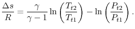
Stagnation pressure is a key variable in propulsion and power
systems. To see why, we examine the relation between stagnation
pressure, stagnation temperature, and entropy. The form of the
combined first and second law that uses enthalpy is
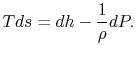 |
(6..8) |
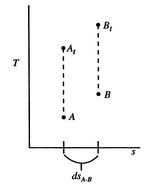
Figure 6.10:
Stagnation and
static states
|
|
This holds for small changes between any thermodynamic states and we
can apply it to a situation in which we consider differences between
stagnation states, say one state having properties
 and
the other having properties
and
the other having properties
 (see
Figure 6.10). The corresponding
static states are also indicated. Because the entropy is the same at
static and stagnation conditions,
(see
Figure 6.10). The corresponding
static states are also indicated. Because the entropy is the same at
static and stagnation conditions,  needs no subscript. Writing
(6.8) in terms of stagnation conditions yields
needs no subscript. Writing
(6.8) in terms of stagnation conditions yields
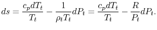
Both sides of the above are perfect differentials and can be
integrated as
For a process with
, the stagnation enthalpy, and hence
the stagnation temperature, is constant. In this situation, the
stagnation pressure is related directly to the entropy as,
 |
(6..9) |
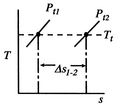
Figure 6.11:
Losses reflected in changes
in stagnation pressure when

|
|
Figure 6.11 shows this relation on
a
-
diagram. We have seen that the entropy is related to the
loss, or irreversibility. The stagnation pressure plays the role of
an indicator of loss if the stagnation temperature is constant. The
utility is that it is the stagnation pressure (and temperature)
which are directly measured, not the entropy. The throttling process
is a representation of flow through inlets, nozzles, stationary
turbomachinery blades, and the use of stagnation pressure as a
measure of loss is a practice that has widespread application.
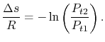
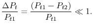
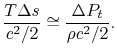
Equation (6.9) can be put in several
useful approximate forms. First, we note that for aerospace
applications we are (hopefully!) concerned with low loss devices, so
that the stagnation pressure change is small compared to the inlet
level of stagnation pressure,
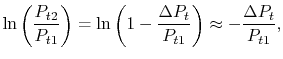
Expanding the logarithm (using
 ),
),
or
Another useful form is obtained by dividing both sides by  and taking the limiting forms of the expression for stagnation
pressure in the limit of low Mach number (
and taking the limiting forms of the expression for stagnation
pressure in the limit of low Mach number ( ). Doing this, we
find:
). Doing this, we
find:
The quantity on the right can be interpreted as the change in the
``Bernoulli constant'' for incompressible (low Mach number) flow.
The quantity on the left is a non-dimensional entropy change
parameter, with the term
 now representing the loss of
mechanical energy associated with the change in stagnation pressure.
now representing the loss of
mechanical energy associated with the change in stagnation pressure.
To summarize:
- For many applications the stagnation temperature is constant and
the change in stagnation pressure is a direct measure of the entropy
increase.
- Stagnation pressure is the quantity that is actually
measured so that linking it to entropy (which is not measured) is
useful.
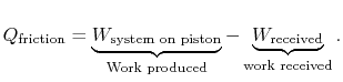
- We can regard the throttling process as a ``free expansion''
at constant temperature
 from the initial stagnation
pressure to the final stagnation pressure. We thus know that, for
the process, the work we need to do to bring the gas back to the
initial state is
from the initial stagnation
pressure to the final stagnation pressure. We thus know that, for
the process, the work we need to do to bring the gas back to the
initial state is
 , which is the ``lost work'' per unit
mass.
, which is the ``lost work'' per unit
mass.
Muddy Points
Why do we find stagnation enthalpy if the velocity never equals zero
in the flow? (MP 6.13)
Why does
remain constant for throttling?
(MP 6.14)
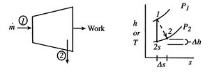
- Adiabatic Efficiency of a Propulsion System Component (Turbine)
Figure 6.12:
Schematic of turbine and
associated thermodynamic representation in  -
coordinates
-
coordinates
|
|
A schematic of a turbine and the accompanying thermodynamic diagram
are given in Figure 6.12. There is a
pressure and temperature drop through the turbine and it produces
work. There is no heat transfer so the expressions that describe
the overall shaft work and the shaft work per unit mass are
If the difference in the kinetic energy at inlet and outlet can be
neglected, Equation (6.11) reduces to
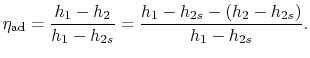
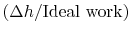
The adiabatic efficiency of the turbine is defined as
The performance of the turbine can be represented
in an
-
plane (similar to a
-
plane for a perfect gas
with constant specific heats) as shown in
Figure 6.12. From the figure the adiabatic
efficiency is
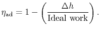
The adiabatic efficiency can therefore be written as
The non-dimensional term
 represents
the departure from isentropic (reversible) processes and hence a
loss. The quantity
represents
the departure from isentropic (reversible) processes and hence a
loss. The quantity  is the enthalpy difference for two
states along a constant pressure line (see diagram). From the
combined first and second laws, for a constant pressure process,
small changes in enthalpy are related to the entropy change by
is the enthalpy difference for two
states along a constant pressure line (see diagram). From the
combined first and second laws, for a constant pressure process,
small changes in enthalpy are related to the entropy change by  , or approximately,
The adiabatic efficiency can thus be approximated as
The quantity
represents a useful figure of merit for
fluid machinery inefficiency due to irreversibility.
Muddy Points
How do you tell the difference between shaft work/power and flow
work in a turbine, both conceptually and mathematically?
(MP 6.15)
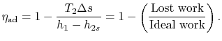
- Isothermal Expansion with Friction
Figure 6.13:
Isothermal
expansion with friction
|
|
In a more general look at the isothermal expansion, we now drop the
restriction to frictionless processes. As seen in
Figure 6.13, work is done to
overcome friction. If the kinetic energy of the piston is
negligible, a balance of forces tells us that
During the expansion, the piston and
the walls of the container will heat up because of the friction. The
heat will be (eventually) transferred to the atmosphere; all
frictional work ends up as heat transferred to the surrounding
atmosphere.
The amount of heat transferred to the atmosphere due to the
frictional work only is thus,
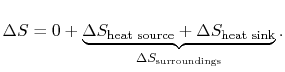
The entropy change of the atmosphere (considered as a heat
reservoir) due to the frictional work is
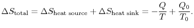
The engine operates in a cycle and the entropy change for the
complete cycle is zero (because entropy is a state variable).
Therefore,
The total entropy change is
Suppose we had an ideal reversible engine working between these same
two temperatures, which extracted the same amount of heat,  , from
the high temperature reservoir, and rejected heat of magnitude
, from
the high temperature reservoir, and rejected heat of magnitude
 to the low temperature reservoir. The work done
by this reversible engine is
to the low temperature reservoir. The work done
by this reversible engine is
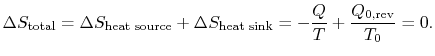
For the reversible engine the total entropy change over a cycle is
Combining the expressions for work and for the entropy changes,
The entropy change for the irreversible cycle can therefore be
written as
The difference in work that the two cycles produce is proportional
to the entropy that is generated during the cycle:
The second law states that the total entropy generated is greater
than zero for an irreversible process, so that the reversible work
is greater than the actual work of the irreversible cycle.
An ``engine effectiveness,''
 , can be defined as
the ratio of the actual work obtained divided by the work that would
have been delivered by a reversible engine operating between the two
temperatures
and
, can be defined as
the ratio of the actual work obtained divided by the work that would
have been delivered by a reversible engine operating between the two
temperatures
and  :
:
The departure from a reversible process is directly reflected in the
entropy change and the decrease in engine effectiveness.
Muddy Points
Why does
 ?
(MP 6.17)
?
(MP 6.17)
In discussing the terms ``closed system'' and ``isolated system,''
can you assume that you are discussing a cycle or not?
(MP 6.18)
Does a cycle process have to have
 ?
(MP 6.19)
?
(MP 6.19)
In a real heat engine, with friction and losses, why is  still 0 if
 ? (MP 6.20)
- Propulsive Power and Entropy Flux
The final example in this section combines a number of ideas
presented in this subject and in Unified in the development of a
relation between entropy generation and power needed to propel a
vehicle.
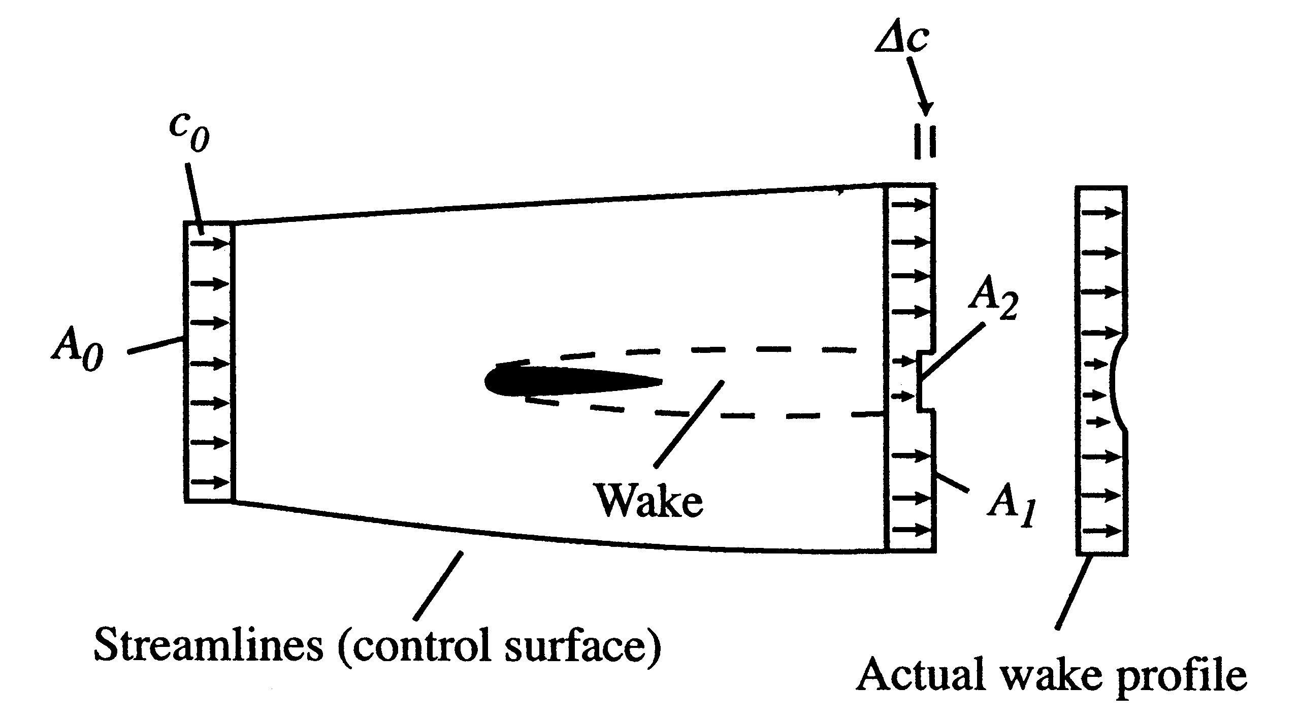
Figure 6.15 shows an aerodynamic shape
(airfoil) moving through the atmosphere at a constant velocity. A
coordinate system fixed to the vehicle has been adopted so that we
see the airfoil as fixed and the air far away from the airfoil
moving at a velocity  . Streamlines of the flow have been
sketched, as has the velocity distribution at station ``0'' far
upstream and station ``d'' far downstream.
. Streamlines of the flow have been
sketched, as has the velocity distribution at station ``0'' far
upstream and station ``d'' far downstream.
The airfoil has a wake, which mixes with the surrounding air and
grows in the downstream direction. The extent of the wake is also
indicated. Because of the lower velocity in the wake the area
between the stream surfaces is larger downstream than upstream.
Figure 6.15:
Airfoil with wake and
control volume for analysis of propulsive power requirement
|
|
We use a control volume description and take the control surface to
be defined by the two stream surfaces and two planes at station 0
and station d. This is useful in simplifying the analysis because
there is no flow across the stream surfaces. The area of the
downstream plane control surface is broken into  , which is the
area outside the wake and
, which is the
area outside the wake and  , which is the area occupied by wake
fluid, i.e., fluid that has suffered viscous losses. The control
surface is also taken far enough away from the vehicle so that the
static pressure can be considered uniform. For fluid which is not in
the wake (no viscous forces), the momentum equation is
, which is the area occupied by wake
fluid, i.e., fluid that has suffered viscous losses. The control
surface is also taken far enough away from the vehicle so that the
static pressure can be considered uniform. For fluid which is not in
the wake (no viscous forces), the momentum equation is
Uniform static pressure therefore implies uniform
velocity, so that on
the velocity is equal to the upstream
value,
. The downstream velocity profile is actually
continuous, as indicated. It is approximated in the analysis as a
step change to make the algebra a bit simpler. (The conclusions
apply to the more general velocity profile as well and we would just
need to use integrals over the wake instead of the algebraic
expressions below.)
The equation expressing mass conservation for the control volume is
 |
(6..12) |
The vertical face of the control surface is far downstream of the
body. By this station, the wake fluid has had much time to mix and
the velocity in the wake is close to the free stream value,
.
We can thus write,
 |
(6..13) |
(We chose our control surface so the condition
 was upheld.)
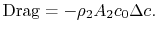
The integral momentum equation (control volume form of the momentum
equation) can be used to find the drag on the vehicle:
 |
(6..14) |
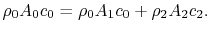
There is no pressure contribution in Eq. (6.14)
because the static pressure on the control surface is uniform. Using
the form given for the wake velocity and expanding the terms in the
momentum equation we obtain
![$\displaystyle \rho_0 A_0 c_0^2 = -\textrm{Drag} +\rho_0 A_1 c_0^2 +\rho_2 A_2[c_0^2 - 2c_0\Delta c + (\Delta c)^2].$](img834.png) |
(6..15) |
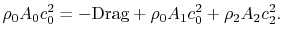
The last term in the right hand side of the momentum equation,
 , is small by virtue of the choice of
control surface and we can neglect it. Doing this and grouping the
terms on the right hand side of Eq. (6.15) in
a different manner, we have
, is small by virtue of the choice of
control surface and we can neglect it. Doing this and grouping the
terms on the right hand side of Eq. (6.15) in
a different manner, we have
The terms in the square brackets on
both sides of this equation are the continuity equation multiplied
by
. They thus sum to zero leaving the curly bracketed terms as
 |
(6..16) |
The wake mass flow is
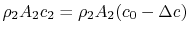 . All this flow has a velocity defect (compared to the free
stream) of
. All this flow has a velocity defect (compared to the free
stream) of  , so that the defect in flux of momentum (the
mass flow in the wake times the velocity defect) is, to first order
in
,
, so that the defect in flux of momentum (the
mass flow in the wake times the velocity defect) is, to first order
in
,
The combined first and second law gives us a means
of relating the entropy and velocity:
The pressure
is uniform ( ) at the downstream station. There is no net shaft
work or heat transfer to the wake so that the mass flux of
stagnation enthalpy is constant. We can also approximate that the
condition of constant stagnation enthalpy holds locally on all
streamlines. Applying both of these to the combined first and second
law yields
) at the downstream station. There is no net shaft
work or heat transfer to the wake so that the mass flux of
stagnation enthalpy is constant. We can also approximate that the
condition of constant stagnation enthalpy holds locally on all
streamlines. Applying both of these to the combined first and second
law yields
For the present situation,  ;
;
 , so that
 |
(6..17) |
In Equation (6.17) the upstream
temperature is used because differences between wake quantities and
upstream quantities are small at the downstream control station. The
entropy can be related to the drag as
 |
(6..18) |
The quantity
 is the entropy flux (mass
flux times the entropy increase per unit mass; in the general case
we would express this by an integral over the locally varying wake
velocity and density). The power needed to propel the vehicle is the
product of
is the entropy flux (mass
flux times the entropy increase per unit mass; in the general case
we would express this by an integral over the locally varying wake
velocity and density). The power needed to propel the vehicle is the
product of
 ,
,
 . From Eq. (6.18), this
can be related to the entropy flux in the wake to yield a compact
expression for the propulsive power needed in terms of the wake
entropy flux:
. From Eq. (6.18), this
can be related to the entropy flux in the wake to yield a compact
expression for the propulsive power needed in terms of the wake
entropy flux:
 |
(6..19) |
This amount of work is dissipated per unit time in connection with
sustaining the vehicle motion. Equation (6.19)
is another demonstration of the relation between lost work and
entropy generation, in this case manifested as power that needs to
be supplied because of dissipation in the wake.
Muddy Points
Is it safe to say that entropy is the tendency for a system to go
into disorder? (MP 6.21)
Douglas Quattrochi
2006-08-06
|


![$\displaystyle \eta_\textrm{ad} = \left[\frac{\textrm{actual work}}
{\textrm{ideal work $(\Delta s=0)$}}\right]_\textrm{for a given
pressure ratio}.$](img799.png)