Assignment 3: Multipole Algorithm
Assigned: 3/14/96
Due: 3/21/96
This assignment may be done in message passing mode or HPF.
It's up to you to write the code the way you wish, and then
tune it for performance.
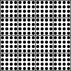
Structure. Imagine dividing a large square into a k by k
grid of cells. Further imagine subdividing each cell into a k by
k grid of bodies also located on a lattice. In other words, there are
 bodies per cell, and
  cells in total
giving a grand total of
  cells. The following example
illustrates this clearly for k = 4. There are
  =
256 bodies with sixteen bodies in each of the sixteen cells.

.gif) calculation:
Pick some random numbers (or your own favorite numbers,
if you do not wish to learn to use the random number
generator)
for the strength of each body, and compute the
potential that each body feels due to the other bodies.
I think the easiest way to do this is
to set a up a (2 dimensional) 3 x
calculation:
Pick some random numbers (or your own favorite numbers,
if you do not wish to learn to use the random number
generator)
for the strength of each body, and compute the
potential that each body feels due to the other bodies.
I think the easiest way to do this is
to set a up a (2 dimensional) 3 x  array
where each column corresponds to a body, and the three
rows contain x, y, and q. You can then make a dynamic
copy which you can cshift around so that everybody
visits everybody.
Alternatively, you can loop through the columns and
spread the information to every other column, by using
the dynamic array to hold the spreaded columns. This
may be slower because of the extra communication
involved.
An approach that take more memory,
but does not require loops is to use
all-to-all broadcasts.
- One level simulation:
Write a program for the following algorithm which is a hybrid fast
multipole method and the direct method. First, compute the three-term
expansion (up to
 ) of each cell. Next compute the
potentials at each point, by combining (a) the results of a direct
computation for points in nearby cells and (b) using the three-term
expansion for points not in nearby cells. (A cell is "nearby"
if it touches at an edge or corner.)
Can you estimate the number of
operations as
 .gif) , i.e. what is
, i.e. what is
 ?
?
- Now implement a "FLIP" operation that turns a multipole expansion into a
three-term local (Taylor) expansion for each cell (up to
 ). What is the operation count for this
routine?
- Modify your program so that you can handle the case where there are
 random points in each box. This means
the location of the body is not centered with respect to the box,
but is located elsewhere.
- Two level simulation:
So far, all we had was one level of cells: the k*k cells.
(Okay, one might say we have two levels, the root representing
the whole structure, and the k*k cells serving as leaves.)
Now we add a level containing k*k/4 cells formed by combing four
of the previous cells into one larger cell. Therefore, what we
have is the root containg the entire grid. The first level is
then a (k/2) x (k/2) division into large cells. (Yes k better
be even.) With 4*k*k bodies per cell. The second division
divides these larger cells into the cells with k*k bodies that
we worked on in parts 1, 2, 3, 4.
The first step is to compute the multipole expansion of each box
at the leaf level. A shift operation combines the multipoles to
the parent node. One can then work down the tree.
I'll leave it to you to decide whether to do the
flipping or just evaluate the multipole expansions
directly.
There are a number of ways to consider implementing this program.
Some ways may be easier to code, and others may run faster. In part
1, you might consider putting the strengths on a two dimensional
array, and look up some fast broadcasting approaches. When learning
to use a parallel machine it is up to you to figure out what runs
fastest. Anyone who has touched a parallel computer knows that
experimenting with different approaches is important.
For question 2, maybe one should use a 3 dimensional array, with the
third axes declared serial (*) and containing the multipole information.
When you step along a serial axis, the data is local to a processor.
Maybe a 5 or 6 dimensional array is more natural, or runs faster, for
the other questions. Should one declare the axes serial (*) ? (Meaning
that the data is local to a processor.)
In your writeup, make sure it is easy to compare the numbers obtained
from the direct method with the various multipole methods. Also make
sure we can compare timings at each level. Run the programs for a few
different k's.
Return to the class home page.

 bodies per cell, and
  cells in total
giving a grand total of
  cells. The following example
illustrates this clearly for k = 4. There are
  =
256 bodies with sixteen bodies in each of the sixteen cells.

.gif) calculation:
Pick some random numbers (or your own favorite numbers,
if you do not wish to learn to use the random number
generator)
for the strength of each body, and compute the
potential that each body feels due to the other bodies.
I think the easiest way to do this is
to set a up a (2 dimensional) 3 x
calculation:
Pick some random numbers (or your own favorite numbers,
if you do not wish to learn to use the random number
generator)
for the strength of each body, and compute the
potential that each body feels due to the other bodies.
I think the easiest way to do this is
to set a up a (2 dimensional) 3 x  array
where each column corresponds to a body, and the three
rows contain x, y, and q. You can then make a dynamic
copy which you can cshift around so that everybody
visits everybody.
 ) of each cell. Next compute the
potentials at each point, by combining (a) the results of a direct
computation for points in nearby cells and (b) using the three-term
expansion for points not in nearby cells. (A cell is "nearby"
if it touches at an edge or corner.)
Can you estimate the number of
operations as
 .gif) , i.e. what is
, i.e. what is
 ?
?
 ). What is the operation count for this
routine?
 random points in each box. This means
the location of the body is not centered with respect to the box,
but is located elsewhere.