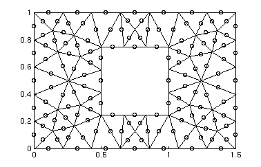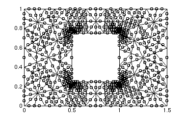


The fine mesh (not shown), contains 525 triangles, 303 linear nodes, and 1131 quadratic nodes.
The mesh is organized in three variables named point, theta, and boundary. The point variable consists of x-y pairs organized in columns for each point in the mesh. The theta matrix contains a colum for each element in the mesh and it provides the six indices one of each of the points in the element. The boundary variable is a single row vector that maps each node in the mesh to a boundary. For each point, the boundary arrray contains a zero (indicating an interior node), or a number between 1 and 8. The top edge (y=1) is 1, the right edge (x=1.5) is 2, the bottom (y=0) is 3, the left edge (x=0) is 4, the top of the cylinder (y=.75) is 5, the right of the cylinder (x=1) is 6, the bottom of the cylinder (y=.25) is 7, and the left of the cylinder (x=.5) is 8.
The file theta2 has the periodic representation of the mesh included in it, i.e. it maps the nodes on the right boundary of the grid to the corresponding node on the left boundary.
Note: there is a file also in the course locker called "plotsolution.m"
This is a matlab .m file and may be used to plot the solution of the stokes
flow problem.
athena% add 2.274
athena% cp /mit/2.274/www/coarse_mesh.mat .
athena% cp /mit/2.274/www/medium_mesh.mat .
athena% cp /mit/2.274/www/fine_mesh.mat .
athean% cp /mit/2.274/www/drawmesh.m .
The above should copy the data file coarse_mesh.mat, medium_mesh.mat, fine_mesh.mat, and the script file drawmesh.m into your local directory. See the instructions below for how to use these files from MATLAB.
>>load coarse_mesh
>>drawmesh( point_coarse, theta_coarse );
>>load medium_mesh
>>drawmesh( point_medium, theta_medium );
The above two lines should produce the plots shown above. If you want to see the node numbering for each of the meshes, then you can use the following command:
>>drawmesh( point_coarse, theta_coarse, boundary_coarse );