An appreciation for the quasistatic approximations will come with a consideration of many case studies. Justification of one or the other of the approximations hinges on using the quasistatic fields to estimate the "error" fields, which are then hopefully found to be small compared to the original quasistatic fields.
In developing any mathematical "theory" for the description of some part of the physical world, approximations are made. Conclusions based on this "theory" should indeed be made with a concern for implicit approximations made out of ignorance or through oversight. But in making quasistatic approximations, we are fortunate in having available the "exact" laws. These can always be used to test the validity of a tentative approximation.
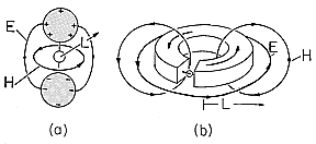
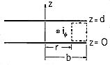
Figure 3.3.1 Prototype systems involving one typical length. (a) EQS system in which source of EMF drives a pair of perfectly conducting spheres having radius and spacing on the order of L. (b) MQS system consisting of perfectly conducting loop driven by current source. The radius of the loop and diameter of its cross-section are on the order of L. Provided that the system of interest has dimensions that are all within a factor of two or so of each other, order of magnitude arguments easily illustrate how the error fields are related to the quasistatic fields. The examples shown in Fig. 3.3.1 are not to be considered in detail, but rather should be regarded as prototypes. The candidate for the EQS approximation in part (a) consists of metal spheres that are insulated from each other and driven by a source of EMF. In the case of part (b), which is proposed for the MQS approximation, a current source drives a current around a one-turn loop. The dimensions are "on the same order" if the diameter of one of the spheres, is within a factor of two or so of the spacing between spheres and if the diameter of the conductor forming the loop is within a similar factor of the diameter of the loop.
If the system is pictured as made up of "perfect conductors" and "perfect insulators," the decision as to whether a quasistatic field ought to be classified as EQS or MQS can be made by a simple rule of thumb: Lower the time rate of change (frequency) of the driving source so that the fields become static. If the magnetic field vanishes in this limit, then the field is EQS; if the electric field vanishes the field is MQS. In reality, materials are not "perfect," neither perfect conductors nor perfect insulators. Therefore, the usefulness of this rule depends on understanding under what circumstances materials tend to behave as "perfect" conductors, and insulators. Fortunately, nature provides us with metals that are extremely good conductors- and with gases, liquids, and solids that are very good insulators- so that this rule is a good intuitive starting point. Chapters 7, 10, and 15 will provide a more mature view of how to classify quasistatic systems.
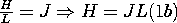
The quasistatic laws are now used in the order summarized by (3.2.5)-(3.2.9) to estimate the field magnitudes. With only one typical length scale L, we can approximate spatial derivatives that make up the curl and divergence operators by~1/L.
ELECTROQUASISTATIC MAGNETOQUASISTATIC Thus, it follows from Gauss' law, (3.2.5a), that typical values of E and are related by
Thus, it follows from Ampère's law, (3.2.5b), that typical values of H and J are related by
As suggested by the integral forms of the laws so far used, these fields and their sources are sketched in Fig. 3.3.1. The EQS laws will predict E lines that originate on the positive charges on one electrode and terminate on the negative charges on the other. The MQS laws will predict lines of H that close around the circulating current.
If the excitation were sinusoidal in time, the characteristic time
for the sinusoidal steady state response would be the reciprocal of the angular frequency
. In any case, if the excitations are time varying, with a characteristic time
the time varying charge implies a current, and this in turn induces an H. We could compute the current in the conductors from charge conservation, (3.2.7a), but because we are interested in the induced H, we use Ampère's law, (3.2.8a), evaluated in the free space region. The electric field is replaced in favor of the charge density in this expression using (1a). the time-varying current implies an H that is time-varying. In accordance with Faraday's law, (3.2.7b), the result is an induced E. The magnetic field intensity is replaced by J in this expression by making use of (1b).
What errors are committed by ignoring the magnetic induction and displacement current terms in the respective EQS and MQS laws?
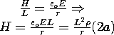
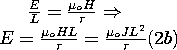
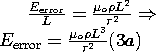
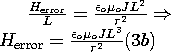
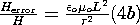
The electric field induced by the quasistatic magnetic field is estimated by using the H field from (2a) to estimate the contribution of the induction term in Faraday's law. That is, the term originally neglected in (3.2.1a) is now estimated, and from this a curl of an error field evaluated. The magnetic field induced by the displacement current represents an error field. It can be estimated from Ampère's law, by using (2b) to evaluate the displacement current that was originally neglected in (3.2.2b). It follows from this expression and (1a) that the ratio of the error field to the quasistatic field is It then follows from this and (1b) that the ratio of the error field to the quasistatic field is
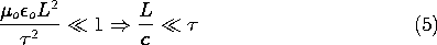
For the approximations to be justified, these error fields must be small compared to the quasistatic fields. Note that whether (4a) is used to represent the EQS system or (4b) is used for the MQS system, the conditions on the spatial scale L and time
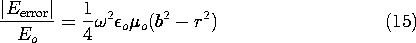
Both the EQS and MQS approximations are predicated on having sufficiently slow time variations (low frequencies) and sufficiently small dimensions so that
where c = 1/
o
o. The ratio L/c is the time required for an electromagnetic wave to propagate at the velocity c over a length L characterizing the system. Thus, either of the quasistatic approximations is valid if an electromagnetic wave can propagate a characteristic length of the system in a time that is short compared to times
If the conditions that must be fulfilled in order to justify the quasistatic approximations are the same, how do we know which approximation to use? For systems modeled by free space and perfect conductors, such as we have considered here, the answer comes from considering the fields that are retained in the static limit (infinite
Recapitulating the rule expressed earlier, consider the pair of spheres shown in Fig. 3.3.1a. Excited by a constant source of EMF, they are charged, and the charges give rise to an electric field. But in this static limit, there is no current and hence no magnetic field. Thus, the static system is dominated by the electric field, and it is natural to represent it as being EQS even if the excitation is time-varying.
Excited by a dc source, the circulating current in Fig. 3.3.1b gives rise to a magnetic field, but there are no charges with attendant electric fields. This time it is natural to use the MQS approximation when the excitation is time varying.
Example 3.3.1. Estimate of Error Introduced by Electroquasistatic
Approximation
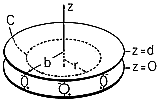
Consider a simple structure fed by a set of idealized sources of EMF as shown in Fig. 3.3.2. Two circular metal disks, of radius b, are spaced a distance d apart. A distribution of EMF generators is connected between the rims of the plates so that the complete system, plates and sources, is cylindrically symmetric. With the understanding that in subsequent chapters we will be examining the underlying physical processes, for now we assume that, because the plates are highly conducting, E must be perpendicular to their surfaces.
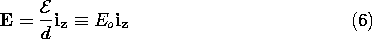
Figure 3.3.2 Plane parallel electrodes having no resistance, driven at their outer edges by a distribution of sources of EMF. The electroquasistatic field laws are represented by (3.2.5a) and (3.2.6a). A simple solution for the electric field between the plates is
where the sign definition of the EMF,
, is as indicated in Fig. 3.3.2. The field of (6) satisfies (3.2.5a) and (3.2.6a) in the region between the plates because it is both irrotational and solenoidal (no charge is assumed to exist in the region between the plates). Further, the field has no component tangential to the plates which is consistent with the assumption of plates with no resistance. Finally, Gauss' jump condition, (1.3.17), can be used to find the surface charges on the top and bottom plates. Because the fields above the upper plate and below the lower plate are assumed to be zero, the surface charge densities on the bottom of the top plate and on the top of the bottom plate are
There remains the question of how the electric field in the neighborhood of the distributed source of EMF is constrained. We assume here that these sources are connected in such a way that they make the field uniform right out to the outer edges of the plates. Thus, it is consistent to have a field that is uniform throughout the entire region between the plates. Note that the surface charge density on the plates is also uniform out to r = b. At this point, (3.2.5a) and (3.2.6a) are satisfied between and on the plates.
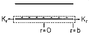
In the EQS order of laws, conservation of charge comes next. Rather than using the differential form, (3.2.7a), we use the integral form, (1.5.2). The volume V is a cylinder of circular cross-section enclosing the lower plate, as shown in Fig. 3.3.3. Because the radial surface current density in the plate is independent of
, integration of J
da on the enclosing surface amounts to multiplying Kr by the circumference, while the integration over the volume is carried out by multiplying
s by the surface area, because the surface charge density is uniform. Thus,
Figure 3.3.3 Parallel plates of Fig. 3.3.2, showing volume containing lower plate and radial surface current density at its periphery. In order to find the magnetic field, we make use of the "secondary" EQS laws, (3.2.8a) and (3.2.9a). Ampère's law in integral form, (1.4.1), is convenient for the present case of high symmetry. The displacement current is z directed, so the surface S is taken as being in the free space region between the plates and having a z-directed normal.
The symmetry of structure and source suggests that H must be
Thus, for this specific configuration, we are at a point in the analysis represented by (2a) in the order of magnitude arguments.
Consider now "higher order" fields and specifically the error committed by neglecting the magnetic induction in the EQS approximation. The correct statement of Faraday's law is (3.2.1a), with the magnetic induction retained. Now that the quasistatic H has been determined, we are in a position to compute the curl of E that it generates.
Again, for this highly symmetric configuration, it is best to use the integral law. Because H is
Figure 3.3.4 Cross-section of system shown in Fig. 3.3.2 showing surface and contour used in evaluating correction E field.
We use the contour shown in Fig. 3.3.4 and assume that the E induced by the magnetic induction is independent of z. Because the tangential E field is zero on the plates, the only contributions to the line integral on the left in (11) come from the vertical legs of the contour. The surface integral on the right is evaluated using (10).
The field at the outer edge is constrained by the EMF sources to be Eo, and so it follows from (12) that to this order of approximation the electric field is
We have found that the electric field at r
b differs from the field at the edge. How big is the difference? This depends on the time rate of variation of the electric field. For purposes of illustration, assume that the electric field is sinusoidally varying with time.
Thus, the time characterizing the dynamics is 1/
Introducing this expression into (13), and calling the second term the "error field," the ratio of the error field and the field at the rim, where r = b, is
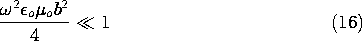
The error field will be negligible compared to the quasistatic field if
for all r between the plates. In terms of the free space wavelength
, defined as the distance an electromagnetic wave propagates at the velocity c = 1/
/
(16) becomes
In free space and at a frequency of 1 MHz, the wavelength is 300 meters. Hence, if we build a circular disk capacitor and excite it at a frequency of 1 MHz, then the quasistatic laws will give a good approximation to the actual field as long as the radius of the disk is much less than 300 meters.
The correction field for a MQS system is found by following steps that are analogous to those used in the previous example. Once the magnetic and electric fields have been determined using the MQS laws, the error magnetic field induced by the displacement current can be found.