Overview of Subject
As illustrated diagrammatically in
Fig. 1.0.1, we start with Maxwell's equations written in integral form.
This chapter begins with a definition of the fields in terms of
forces and
sources followed by a review of each of the integral laws. Interwoven
with the development are examples intended to develop the methods for
surface and volume integrals used in stating the
laws. The examples are also intended to attach at least one physical
situation to each of the laws. Our objective in the chapters that
follow is to make these laws useful, not only in modeling engineering
systems but in dealing with practical systems in a qualitative
fashion (as an inventor often does). The integral laws are directly
useful for (a) dealing with fields in this qualitative way, (b)
finding fields in simple configurations having a great deal of
symmetry, and (c) relating fields to their sources.
Chapter 2 develops a differential description from the integral laws.
By following the examples and some of the homework
associated with each of the sections, a minimum background in the
mathematical theorems and operators is developed. The differential
operators and associated integral theorems are brought in as needed.
Thus, the divergence and curl operators, along with the theorems of
Gauss and Stokes, are developed in Chap. 2, while the gradient operator
and integral theorem are naturally derived in Chap. 4.
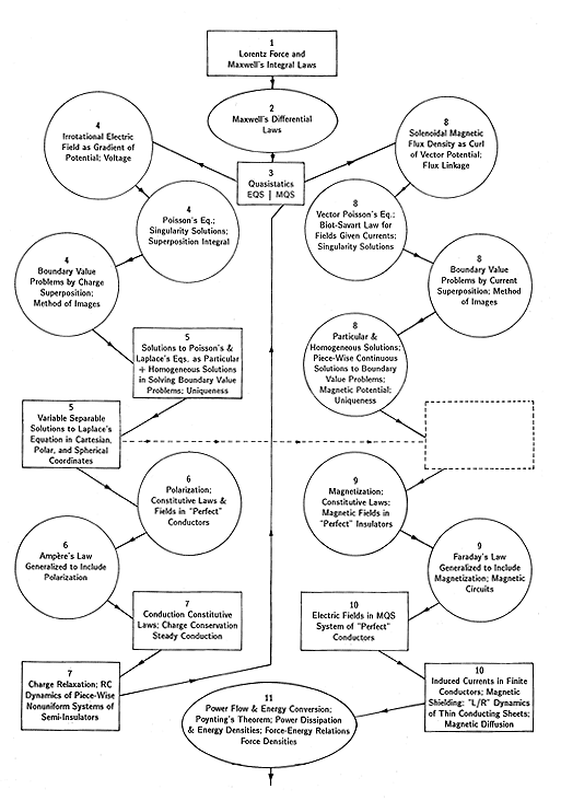
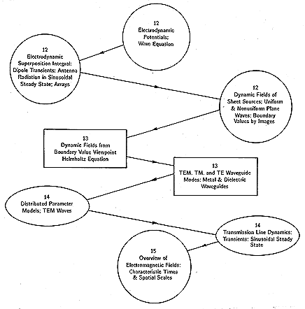 Figure 1.0.1 Outline of Subject. The three columns, respectively for electroquasistatics, magnetoquasistatics and electrodynamics, show parallels in development.
Static fields are often the first topic in developing an
understanding of phenomena predicted by Maxwell's equations. Fields
are not measurable, let alone of practical interest, unless they are
dynamic. As developed here, fields are never truly static. The
subject of quasistatics, begun in Chap. 3, is central to the approach
we will use to understand the implications of Maxwell's equations.
A mature understanding of these equations is achieved when one has
learned how to neglect complications that are inconsequential. The
electroquasistatic (EQS) and magnetoquasistatic (MQS) approximations
are justified if time rates of change are slow enough
(frequencies are low enough) so that time delays due to the propagation
of electromagnetic waves are unimportant. The examples considered in
Chap. 3 give some notion as to which of the two approximations is
appropriate in a given situation. A full appreciation for the
quasistatic approximations will come into view as the EQS and MQS
developments are drawn together in Chaps. 11 through 15.
Although capacitors and inductors are examples in
the electroquasistatic and magnetoquasistatic categories,
respectively, it is not true that quasistatic systems can be generally
modeled by frequency-independent circuit elements. High-frequency
models for transistors are correctly based on the EQS approximation.
Electromagnetic wave delays in the transistors are not consequential.
Nevertheless, dynamic effects are important and the
EQS approximation can contain the finite time for charge
migration. Models for eddy current shields or
heaters are correctly based on the MQS approximation. Again, the
delay time of an electromagnetic wave is unimportant while the
all-important diffusion time of the magnetic field is represented by
the MQS laws. Space charge waves on an electron beam or spin waves in
a saturated magnetizable material are often described by EQS and MQS
laws, respectively, even though frequencies of interest are in the
GHz range.
The parallel developments of EQS (Chaps. 4-7) and MQS systems
(Chaps. 8-10) is emphasized by the first page of Fig. 1.0.1. For
each topic in the EQS
column to the left there is an analogous one at the same level in the
MQS column. Although the field concepts and mathematical
techniques used in dealing with EQS and MQS systems are often similar,
a comparative study reveals as many contrasts as direct analogies.
There is a two-way interplay between the electric and magnetic
studies. Not only are results from the EQS developments applied in the
description of MQS systems, but the examination of MQS situations
leads to a greater appreciation for the EQS laws.
At the tops of the EQS and the MQS columns, the first page of Fig.
1.0.1,
general (contrasting) attributes of the electric and magnetic fields
are identified. The developments then lead from
situations where the field sources are prescribed to where they are to
be determined. Thus, EQS electric fields are first found from
prescribed distributions of charge, while MQS magnetic fields are
determined given the currents. The development of the EQS field
solution is a direct
investment in the subsequent MQS derivation. It is then recognized
that in many practical situations, these sources are induced in
materials and must therefore be found as part of the field solution.
In the first of these situations, induced sources are on the
boundaries of conductors having a sufficiently high electrical
conductivity to be modeled as "perfectly" conducting. For the EQS
systems, these sources are surface charges, while for the MQS, they are
surface currents. In either case, fields must satisfy boundary
conditions, and the EQS study provides not only mathematical
techniques but even partial differential equations directly
applicable to MQS problems.
Polarization and magnetization account for field sources that can
be prescribed (electrets and permanent magnets) or induced by the
fields themselves. In the Chu formulation used here, there is a
complete analogy between the way in which polarization and
magnetization are represented. Thus, there is a direct transfer of
ideas from Chap. 6 to Chap. 9.
The parallel quasistatic studies culminate in Chaps. 7 and 10 in an
examination of loss phenomena. Here we learn that very different
answers must be given to the question "When is a conductor
perfect?" for EQS on one hand, and MQS on the other.
In Chap. 11, many of the concepts developed previously are put to
work through the consideration of the flow of power, storage of
energy, and production of electromagnetic forces. From this chapter
on, Maxwell's equations are used without approximation. Thus, the
EQS and MQS approximations are seen to represent systems in which
either the electric or the magnetic energy storage dominates
respectively.
In Chaps. 12 through 14, the focus is on electromagnetic waves. The
development is a natural extension of the approach taken in the EQS
and MQS columns. This is emphasized by the outline represented on
the right page of Fig. 1.0.1. The topics of Chaps. 12 and 13
parallel those of the EQS and MQS columns on the previous page.
Potentials used to represent electrodynamic fields are a natural
generalization of those used for the EQS and MQS systems. As for the
quasistatic fields, the fields of given sources are considered first.
An immediate practical application is therefore the description of
radiation fields of antennas.
The boundary value point of view, introduced for EQS systems in Chap.
5 and for MQS systems in Chap. 8, is the basic theme of Chap. 13.
Practical examples include simple transmission lines and waveguides.
An understanding of transmission line dynamics, the subject of Chap. 14,
is necessary in dealing with the "conventional" ideal
lines that model most high-frequency systems. They are also
shown to provide useful models for representing quasistatic dynamical
processes.
To make practical use of Maxwell's equations, it is necessary to
master the art of making approximations. Based on the
electromagnetic properties and dimensions of a system and on the time
scales (frequencies) of importance, how can a physical system be
broken into electromagnetic subsystems, each described by its
dominant physical processes? It is with this goal in mind that the
EQS and MQS approximations are introduced in Chap. 3, and to this
end that Chap. 15 gives an overview of electromagnetic fields.

