1.1
The Lorentz Law in Free Space

There are two points of view for formulating a theory of electrodynamics. The older one views the forces of attraction or repulsion between two charges or currents as the result of action at a distance. Coulomb's law of electrostatics and the corresponding law of magnetostatics were first stated in this fashion. Faraday^[1] introduced a new approach in which he envisioned the space between interacting charges to be filled with fields, by which the space is activated in a certain sense; forces between two interacting charges are then transferred, in Faraday's view, from volume element to volume element in the space between the interacting bodies until finally they are transferred from one charge to the other. The advantage of Faraday's approach was that it brought to bear on the electromagnetic problem the then well-developed theory of continuum mechanics. The culmination of this point of view was Maxwell's formulation^[2] of the equations named after him.

From Faraday's point of view, electric and magnetic fields are defined at a point r even when there is no charge present there. The fields are defined in terms of the force that would be exerted on a test charge q if it were introduced at r moving at a velocity v at the time of interest. It is found experimentally that such a force would be composed of two parts, one that is independent of v, and the other proportional to v and orthogonal to it. The force is summarized in terms of the electric field intensity E and magnetic flux density _oH by the Lorentz force law. (For a review of vector operations, see Appendix 1.)

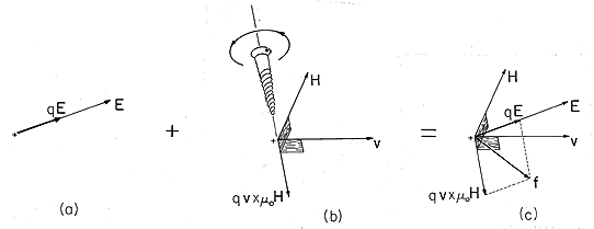
Figure 1.1.1 Lorentz force f in geometric relation to the electric and magnetic field intensities, E and H, and the charge velocity v: (a) electric force, (b) magnetic force, and (c) total force.

The superposition of electric and magnetic force contributions to (1) is illustrated in Fig. 1.1.1. Included in the figure is a reminder of the right-hand rule used to determine the direction of the cross-product of v and _o H. In general, E and H are not uniform, but rather are functions of position r and time t: E = E (r, t) and _oH = _oH (r, t).

In addition to the units of length, mass, and time associated with mechanics, a unit of charge is required by the theory of electrodynamics. This unit is the coulomb. The Lorentz force law, (1), then serves to define the units of E and of _oH.

We can only establish the units of the magnetic flux density _oH from the force law and cannot argue until Sec. 1.4 that the derived units of H are ampere/meter and hence of _o are henry/meter.

In much of electrodynamics, the predominant concern is not with mechanics but with electric and magnetic fields in their own right. Therefore, it is inconvenient to use the unit of mass when checking the units of quantities. It proves useful to introduce a new name for the unit of electric field intensity- the unit of volt/meter.

In the summary of variables given in Table 1.8.2 at the end of the chapter, the fundamental units are SI, while the derived units exploit the fact that the unit of mass, kilogram = volt-coulomb-second²/meter² and also that a coulomb/second = ampere. Dimensional checking of equations is guaranteed if the basic units are used, but may often be accomplished using the derived units. The latter communicate the physical nature of the variable and the natural symmetry of the electric and magnetic variables.

Example 1.1.1. Electron Motion in Vacuum in a Uniform Static Electric Field

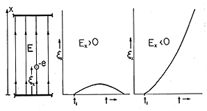
In vacuum, the motion of a charged particle is limited only by its own inertia. In the uniform electric field illustrated in Fig. 1.1.2, there is no magnetic field, and an electron starts out from the plane x = 0 with an initial velocity v_i.

Figure 1.1.2 An electron, subject to the uniform electric field intensity E_x, has the position _x, shown as a function of time for positive and negative fields.

The "imposed" electric field is E = i_x E_x, where i_x is the unit vector in the x direction and E_x is a given constant. The trajectory is to be determined here and used to exemplify the charge and current density in Example 1.2.1.

With m defined as the electron mass, Newton's law combines with the Lorentz law to describe the motion.

The electron position _x is shown in Fig. 1.1.2. The charge of the electron is customarily denoted by e (e = 1.6 x 10^-19 coulomb) where e is positive, thus necessitating an explicit minus sign in (4).

By integrating twice, we get

where c₁ and c₂ are integration constants. If we assume that the electron is at _x = 0 and has velocity v_i when t = t_i, it follows that these constants are

Thus, the electron position and velocity are given as a function of time by

With x defined as upward and E_x > 0, the motion of an electron in an electric field is analogous to the free fall of a mass in a gravitational field, as illustrated by Fig. 1.1.2. With E_x < 0, and the initial velocity also positive, the velocity is a monotonically increasing function of time, as also illustrated by Fig. 1.1.2.

Example 1.1.2. Electron Motion in Vacuum in a Uniform Static Magnetic Field

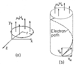
The magnetic contribution to the Lorentz force is perpendicular to both the particle velocity and the imposed field. We illustrate this fact by considering the trajectory resulting from an initial velocity v_iz along the z axis. With a uniform constant magnetic flux density _oH existing along the y axis, the force is

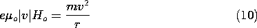
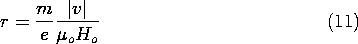
The cross-product of two vectors is perpendicular to the two vector factors, so the acceleration of the electron, caused by the magnetic field, is always perpendicular to its velocity. Therefore, a magnetic field alone cannot change the magnitude of the electron velocity (and hence the kinetic energy of the electron) but can change only the direction of the velocity. Because the magnetic field is uniform, because the velocity and the rate of change of the velocity lie in a plane perpendicular to the magnetic field, and, finally, because the magnitude of v does not change, we find that the acceleration has a constant magnitude and is orthogonal to both the velocity and the magnetic field. The electron moves in a circle so that the centrifugal force counterbalances the magnetic force. Figure 1.1.3a illustrates the motion. The radius of the circle is determined by equating the centrifugal force and radial Lorentz force

Figure 1.1.3 (a) In a uniform magnetic flux density _oH_o and with no initial velocity in the y direction, an electron has a circular orbit. (b) With an initial velocity in the y direction, the orbit is helical.

which leads to

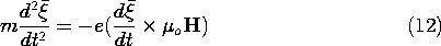
The foregoing problem can be modified to account for any arbitrary initial angle between the velocity and the magnetic field. The vector equation of motion (really three equations in the three unknowns _x, _y, _z)

is linear in , and so solutions can be superimposed to satisfy initial conditions that include not only a velocity v_iz but one in the y direction as well, v_iy. Motion in the same direction as the magnetic field does not give rise to an additional force. Thus, the y component of (12) is zero on the right. An integration then shows that the y directed velocity remains constant at its initial value, v_iy. This uniform motion can be added to that already obtained to see that the electron follows a helical path, as shown in Fig. 1.1.3b.

It is interesting to note that the angular frequency of rotation of the electron around the field is independent of the speed of the electron and depends only upon the magnetic flux density, _o H_o. Indeed, from (11) we find

For a flux density of 1 volt-second/meter (or 1 tesla), the cyclotron frequency is f_c = _c/2 = 28 GHz. (For an electron, e = 1.602 x 10^-19 coulomb and m = 9.106 x 10^-31 kg.) With an initial velocity in the z direction of 3 x 10⁷ m/s, the radius of gyration in the flux density _o H = 1 tesla is r = v_iz/_c = 1.7 x 10^-4 m.