10.6
Magnetic Diffusion Transient Response

The self-consistent distribution of current density and magnetic field intensity in the volume of a uniformly conducting material is determined from the laws given in Sec. 10.5 and summarized by the magnetic diffusion equation (10.5.8). In this section, we illustrate magnetic diffusion phenomena by considering the transient that results when a current is abruptly turned on or off.

In contrast to Laplace's equation, the diffusion equation involves a time rate of change, and so it is necessary to deal with the time dependence in much the same way as the space dependence. The diffusion process considered in this section is in one spatial dimension, with time as the second "dimension." Our approach builds on product solutions and the solution of boundary value problems by superposition, as introduced in Chap. 5.

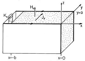
Figure 10.6.1 A block of uniformly conducting material having length b and thickness a is sandwiched between perfectly conducting electrodes that are driven along their edges at x = -b by a distributed current source. Current density and field intensity in the block are, respectively, y and z directed, each depending on (x, t).

The class of configurations of interest is illustrated in Fig. 10.6.1. Perfectly conducting electrodes are driven along their edges at x = -b by a distributed current source. The uniformly conducting material is sandwiched between these electrodes. The current originating in the source then circulates in the x direction through the electrode in the y = 0 plane to a point where it passes in the y direction through the conducting material. It is then returned to the source through the other perfectly conducting plate. Note that this configuration is a special case of that shown in Fig. 10.5.1, where the current density is transverse to a magnetic field intensity that has only one component, H_z.

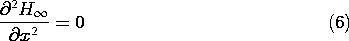
If this field and the associated current density are indeed independent of y, then it follows from (10.5.10) and (10.5.11) that H_z satisfies the one-dimensional diffusion equation

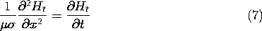
and the only component of the current density is related to H_z by Ampère's law

Note that this one-dimensional model correctly requires that the current density, and hence the electric field intensity, be normal to the perfectly conducting electrodes at y = 0 and y = a.

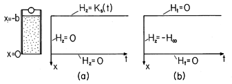
The distributed current source, perfectly conducting sheets and conducting block form a closed path for currents that circulate in x - y planes. These extend to infinity in the + and -z directions in the manner of an infinite one-turn solenoid. The field outside the outermost of these current paths is therefore taken as being zero. Ampère's continuity condition then requires that at the surface x = -b, where the distributed current source is located, the enclosed magnetic field intensity be equal to the imposed surface current density K_s. In the plane x = 0, the situation is similar except that there is no surface current density, and so the magnetic field intensity must be zero. Thus, consistent with solving a differential equation that is second order in x, are the two boundary conditions

The equation is first order in its time dependence, suggesting that to complete the specification of the transient solution, the initial value of H_z must also be given.

Figure 10.6.2 Boundary and initial conditions for one-dimensional magnetic diffusion pictured in the x - t plane. (a) The total fields at the ends of the block are constrained to be equal to the driving surface current density and to zero, respectively, while there is one initial condition when t = 0. (b) The transient part of the solution is zero at the boundaries and satisfies the initial condition that makes the total solution assume the current value when t = 0.

It is helpful to picture the boundary and initial conditions needed to uniquely specify solutions to (2) in the x - t plane, as shown in Fig. 10.6.2a. Here the conducting block can be pictured as extending from x = 0 to x = -b, with the field between a function of x that evolves in the t "direction." Presumably, the distribution of H_z in the x - t space is predicted by (1) with the boundary conditions of (3) at x = 0 and x = -b and the initial condition of (4) when t = 0.

Is the solution for H_z (t) uniquely specified by (1), the boundary conditions of (3), and the initial condition of (4)? A proof that it is can be made following a line of reasoning suggested by the EQS uniqueness arguments of Sec. 7.8.

Suppose that the drive is a step function of time, so that the final state is one of uniform steady conduction. Then, the linearity of (1) makes it possible to think of the total field as being the superposition of this steady field and a transient part.

The steady solution, which presumably prevails as t , satisfies (1) with the time derivative set equal to zero,

while the transient part satisfies the complete equation.

Because the steady solution satisfies the boundary conditions for all time t > 0, the boundary conditions satisfied by the transient part are homogeneous.

However, the steady solution does not satisfy the initial condition. The transient solution is therefore adjusted so that the total solution does.

The conditions satisfied by the transient part of the solution on the boundaries in the x - t space are pictured in Fig. 10.6.2b.

Product Solutions to the One-Dimensional Diffusion Equation

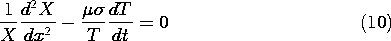
The approach now used to find the H_t that satisfies (7) and the conditions of (8) and (9) is familiar from finding Cartesian coordinate product solutions to Laplace's equation in two dimensions in Sec. 5.4. Here the second "dimension" is t and we consider solutions that take the form H_t = X(x) T(t). Substitution into (7) and division by XT gives

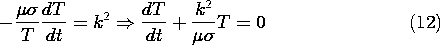
With the first term taken as -k² and the second as k², it follows that

and

Given the boundary conditions of (8), the appropriate solution to (11) is

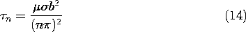
where n can be any integer. Associated with each of these modes is a time dependence given by (12) as a decaying exponential with the time constant

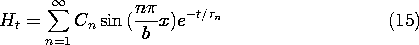
Thus, we are led to a transient part of the solution that is itself a superposition of modes, each satisfying the boundary conditions.

When t = 0, the modes take the form of a Fourier series. Thus, the coefficients C_n can be used to satisfy the initial condition, (9).

In the following example, the coefficients are evaluated for specific initial conditions. However, because the "short time" and "long time" field and current distributions are known at the outset, much of the dynamics can be anticipated at the outset. For times that are very short compared to the magnetic diffusion time b², the conducting block must act as a perfect conductor. In this short time limit, we know from Chap. 8 that the current from the distributed source is confined to the surface at x = -b. Thus, for early times, the distribution represented by the series of (15) tends to be an impulse function of x. After many magnetic diffusion times, the current reaches a steady state and achieves a distribution that would be predicted in the first half of Chap. 7. The following example fills in the evolution from the field of a perfectly conducting system to that for steady conduction.

Example 10.6.1. Response to a Step in Current

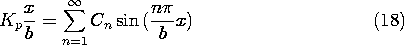
When t = 0, suppose that there are no currents or associated fields. Then the current source suddenly becomes the constant K_p. The solution to (6) that is zero at x = 0 and is K_p at x = -b is

This is the field associated with a constant current density K_p/b that is uniformly distributed over the cross-section of the block. Because there is no initial magnetic field, it follows from (9) that the initial transient part of the field must cancel the steady part.

This must be the distribution of H_t given by (15) when t = 0.

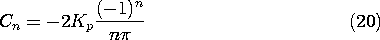
Following the procedure familiar from Sec. 5.5, the coefficients C_n are now evaluated by multiplying both sides of this expression by sin (m /b), multiplying by dx, and integrating from x = -b to x = 0.

From the series on the right, only the term m = n is not zero. Carrying out the integration on the left

---

³ sin (u) udu = sin (u) - u cos (u) then gives an expression that can be solved for C_m. Replacing m n then gives

Finally, (16) and (15) [the latter evaluated using (20)] are superimposed as required by (5) to give the desired description of how the field evolves as a function of space and time.

The distribution of current density follows from this expression substituted into Ampère's law, (2).

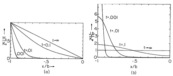
Figure 10.6.3 (a) Distribution of H_z in the conducting block of Fig. 10.6.1 in response to applying a step in current with no initial field. In terms of time normalized to the magnetic diffusion time based on the length b, the field diffuses into the block, finally assuming the linear distribution expected for steady conduction. (b) Distribution of J_y with normalized time as a parameter. The initial distribution is an impulse (a surface current density) at x = -b, while the final distribution is uniform.

These expressions are pictured in Fig. 10.6.3. Note that the higher the order of a term, the more rapid its exponential decay with time. As a result, the most terms in the series are needed when t = 0⁺. These are needed to make the initial magnetic field intensity zero and the initial current density an impulse at x = -b. Because the lowest mode in the transient part of either H_z or J_y has the longest time constant, the long-time response is dominated by the steady response and the first term in the series. Of course, with the decay of the transient part, the field approaches a linear x dependence while the current density assumes the uniform distribution expected for a steady current.