The objective in this section is to derive a statement of energy
conservation from Maxwell's equations in the form identified in Sec.
11.1. The conservation theorem includes the effects of both
displacement current and of magnetic induction. The EQS and MQS
limits, respectively, can be taken by neglecting those terms having
their origins in the magnetic induction 
 o (H + M)/
t on the one hand, and in the displacement current density (
o (H + M)/
t on the one hand, and in the displacement current density ( o
E + P)/ t on the other.
o
E + P)/ t on the other.
Ampère's law, including the effects of polarization, is (11.0.2).

Faraday's law, including the effects of magnetization, is (11.0.3).

These field-theoretical laws play a role analogous to that of
the circuit equations in the introductory section. What we
do next is also analogous. For the circuit case, we form
expressions that are quadratic in the dependent variables. Several
considerations guide the following manipulations. One aim is to
derive an expression involving power dissipation or conversion
densities and time rates of change of energy storages. The power per
unit volume imparted to the current density of unpaired charge
follows directly from the Lorentz force law (at least in free space).
The force on a particle of charge q is

The rate of work on the particle is

If the particle density is N and only one species of charged
particles exists, then the rate of work per unit volume
is

Thus, one must anticipate that an energy conservation law that
applies to free space must contain the term Ju  E.
In order to obtain this term, one should dot multiply (1) by E.
E.
In order to obtain this term, one should dot multiply (1) by E.
A second consideration that motivates the form of the energy
conservation law is the aim to obtain a perfect divergence of density
of power flow. Dot multiplication of (1) by E generates ( x H) E. This term is made into a perfect
divergence if one adds to it -( x E) H,
i.e., if one subtracts (2) dot multiplied by H.
x H) E. This term is made into a perfect
divergence if one adds to it -( x E) H,
i.e., if one subtracts (2) dot multiplied by H.
Indeed,

Thus, subtracting (2) dot multiplied by H from (1) dot multiplied
by E one obtains

In writing the first and third terms on the right, we have exploited
the relation u du = d( u2). These two
terms now take the form of the energy storage term in the power
theorem, (11.1.3). The desire to obtain expressions taking this form
is a third consideration
contributing to the choice of ways in which (1) and (2) were combined.
We could have seen at the outset that dotting E with (1) and
subtracting (2) after it had been dotted with H would result in
terms on the right taking the desired form of "perfect" time
derivatives.
u2). These two
terms now take the form of the energy storage term in the power
theorem, (11.1.3). The desire to obtain expressions taking this form
is a third consideration
contributing to the choice of ways in which (1) and (2) were combined.
We could have seen at the outset that dotting E with (1) and
subtracting (2) after it had been dotted with H would result in
terms on the right taking the desired form of "perfect" time
derivatives.
In the electroquasistatic limit, the magnetic induction terms on
the right in Faraday's law, (2), are neglected. It follows from the
steps leading to (7) that in the EQS approximation, the third and
fourth terms on the right of (7) are negligible. Similarly, in the
magnetoquasistatic limit, the displacement current, the last two terms
on the right in Ampère's law, (1), is neglected. This implies that
for MQS systems, the first two terms on the right in (7) are
negligible.
Systems Composed of Perfect Conductors and Free Space
Quasistatic
examples in this category are the EQS systems of Chaps. 4 and 5 and
the MQS systems of Chap. 8, where perfect conductors are surrounded by
free space. Whether quasistatic or electrodynamic, in these
configurations, P = 0, M = 0; and where there is a
current density Ju, the perfect conductivity insures that
E = 0. Thus, the second and last two terms on the right in (7)
are zero. For perfect conductors surrounded by free space, the
differential form of the power theorem becomes
with

and

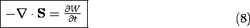
where S is the Poynting vector and W is the sum
of the electric and magnetic energy densities. The electric and
magnetic fields are confined to the free space regions. Thus, power
flow and energy storage pictured in terms of these variables occur
entirely in the free space regions.
Limiting cases governed by the EQS and MQS laws, respectively, are
distinguished by having predominantly electric and magnetic energy
densities. The following simple examples illustrate the application of
the power theorem to two simple quasistatic situations. Applications
of the theorem to electrodynamic systems will be taken up in Chap. 12.
Example 11.2.1. Plane Parallel Capacitor
The plane parallel capacitor of Fig. 11.2.1 is familiar from
Example 3.3.1. The circular electrodes are perfectly conducting,
while the region between the electrodes is free space. The system is
driven by a voltage
source distributed around the edges of the electrodes. Between the
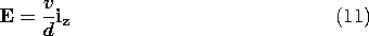
electrodes, the electric field is simply the voltage
divided by the plate spacing (3.3.6),
while the magnetic field that follows from the integral form of Ampère's
law is (3.3.10).
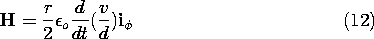
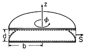 Figure 11.2.1 Plane parallel circular electrodes
are driven by a distributed voltage source. Poynting flux through
surface denoted by dashed lines accounts for rate of change of
electric energy stored in the enclosed volume.
Figure 11.2.1 Plane parallel circular electrodes
are driven by a distributed voltage source. Poynting flux through
surface denoted by dashed lines accounts for rate of change of
electric energy stored in the enclosed volume.
Consider the application of the integral version of (8) to the
surface S enclosing the
region between the electrodes in Fig. 11.2.1. First we determine the
power flowing into the volume through this surface by evaluating the
left-hand side of (8). The density of power flow follows from (11)
and (12).

The top and bottom surfaces have normals perpendicular to this
vector, so the only contribution comes from the surface at r = b.
Because S is constant on that surface, the integration amounts to
a multiplication.

where

Here the expression has been written as the rate of change of the
energy stored in the capacitor. With E again given by (11), we
double-check the expression for the time rate of change of energy
storage.

From the field viewpoint, power flows into the volume through the
surface at r = b and is stored in the form of electrical energy in the
volume between the plates. In the quasistatic approximation used to
evaluate the electric field, the magnetic energy storage is neglected
at the outset because it is small compared to the electric energy
storage. As a check on the implications of this approximation,
consider the total magnetic energy storage. From (12),

Comparison of this expression with the electric energy storage found
in (15) shows that the EQS approximation is valid provided that
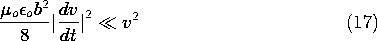
For a sinusoidal excitation of frequency  , this gives
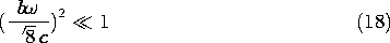
where c is the free space velocity of light (3.1.16). The
result is familiar from Example 3.3.1. The requirement that the
propagation time b/c of an electromagnetic wave be short compared to a
period 1/ is equivalent to the requirement that the magnetic
energy storage be negligible compared to the electric energy storage.
A second example offers the opportunity to apply the integral
version of (8) to a simple MQS system.
Example 11.2.2. Long Solenoidal Inductor
The perfectly conducting one-turn solenoid of Fig. 11.2.2 is
familiar from Example 10.1.2. In terms of the terminal current i =
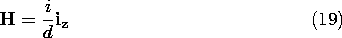
Kd, the magnetic field intensity inside is (10.1.14),
while the electric field is the sum of the particular and conservative
homogeneous parts [(10.1.15) for the particular part and Eh
for the conservative part].

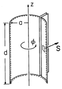 Figure 11.2.2 One-turn solenoid
surrounding volume enclosed by surface S denoted by dashed lines.
Poynting flux through this surface accounts for the rate of change of
magnetic energy stored in the enclosed volume.
Figure 11.2.2 One-turn solenoid
surrounding volume enclosed by surface S denoted by dashed lines.
Poynting flux through this surface accounts for the rate of change of
magnetic energy stored in the enclosed volume.
Consider how the power flow through the surface S of the volume
enclosed by the coil is accounted for by the time rate of change of
the energy stored. The Poynting flux implied by (19) and (20) is

This Poynting vector has no component normal to the top and bottom
surfaces of the volume. On the surface at r = a, the first term in
brackets is constant, so the
integration on S amounts to a multiplication by the area. Because
Eh is irrotational, the integral of Eh ds =
E h rd around a contour at r = a must be zero. For
this reason, there is no net contribution of Eh to the surface
integral.
h rd around a contour at r = a must be zero. For
this reason, there is no net contribution of Eh to the surface
integral.

where

Here the result shows that the power flow is accounted for by the
rate of change of the stored magnetic energy. Evaluation of the right
hand side of (8), ignoring the electric energy storage, indeed gives
the same result.

The validity of the quasistatic approximation is examined by comparing
the magnetic energy storage to the neglected electric energy storage.
Because we are only interested in an order of magnitude comparison and
we know that the homogeneous solution is proportional to the
particular solution (10.1.21), the latter can be approximated by the
first term in (20).

We conclude that the MQS approximation is valid provided that the
angular frequency is small compared to the time required for an
electromagnetic wave to propagate the radius a of the solenoid and
that this is equivalent to having an electric energy storage that is
negligible compared to the magnetic energy storage.

A note of caution is in order. If the gap between the
"sheet" terminals is made very small, the electric energy storage
of the homogeneous part of the E field can become large. If it
becomes comparable to the magnetic energy storage, the structure
approaches the condition of resonance of the circuit consisting of
the gap capacitance and solenoid inductance. In this limit, the MQS
approximation breaks down. In practice, the electric energy stored
in the gap would be dominated by that in the connecting plates, and
the resonance could be described as the coupling of MQS and EQS
systems as in Example 3.4.1.
In the following sections, we use (7) to study the storage and
dissipation of energy in macroscopic media.

