11.3
Ohmic Conductors With Linear Polarization andMagnetization

Consider a stationary material described by the constitutive laws

where the susceptibilities _e and _m, and hence the permittivity and permeability and , as well as the conductivity , are all independent of time. Expressed in terms of these constitutive laws for P and M, the polarization and magnetization terms in (11.2.7) become

Because these terms now appear in (11.2.7) as perfect time derivatives, it is clear that in a material having "linear" constitutive laws, energy is stored in the polarization and magnetization processes.

With the substitution of these terms into (11.2.7) and Ohm's law for J_u, a conservation law is obtained in the form discussed in Sec. 11.1. For an electrically and magnetically linear material that obeys Ohm's law, the integral and differential conservation laws are (11.1.1) and (11.1.3), respectively, with

The power flux density S and the energy density W appear as in the free space conservation theorem of Sec. 11.2. The energy storage in the polarization and magnetization is included by simply replacing the free space permittivity and permeability by and , respectively.

The term P_d is always positive and seems to represent a rate of power loss from the electromagnetic system. That P_d indeed represents power converted to thermal form is motivated by considering the origins of the Ohmic conduction law. In terms of the bipolar conduction model introduced in Sec. 7.1, positive and negative carriers, respectively, experience the forces f₊ and f_-. These forces are balanced by collisions with the surrounding particles, and hence the work done by the field in forcing the migration of the particles is converted into thermal energy. If the velocity of the families of particles are, respectively, v₊ and v_-, and the number densities N₊ and N_-, respectively, then the rate of work performed on the carriers (per unit volume) is

In recognition of the balance between collision forces and electrical forces, the forces of (4) are replaced by |q₊|E and -|q_-|E, respectively.

If, in turn, the velocities are written as the products of the respective mobilities and the macroscopic electric field, (7.1.3), it follows that

where the definition of the conductivity (7.1.7) has been used.

The power dissipation density P_d = E E (watts/m³) represents a rate of energy loss from the electromagnetic system to the thermal system.

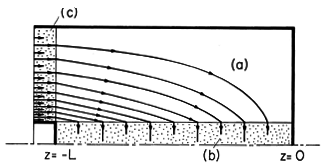
Example 11.3.1. The Poynting Vector of a Stationary Current Distribution

In Example 7.5.2, we studied the electric fields in and around a circular cylindrical conductor fed by a battery in parallel with a disk-shaped conductor. Here we determine the Poynting vector field and explore its spatial relationship to the dissipation density.

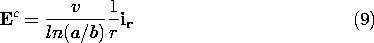
First, within the circular cylindrical conductor [region (b) in Fig. 11.3.1], the electric field was found to be uniform, (7.5.7),

while in the surrounding free space region, it was [from (7.5.11)]

and in the disk-shaped conductor [from (7.5.9)]

By symmetry, the magnetic field intensity is directed. The component of H is most easily evaluated from the integral form of Ampère's law. The current density in the circular conductor follows from (7) as J_o = v/L. Then,

The magnetic field distribution in the disk conductor is also deduced from Ampère's law. In this region, it is easiest to evaluate the r component of Ampère's differential law with the current density J^c = E^c, with E^c given by (9). Integration of this partial differential equation on z then gives a linear function of z plus an "integration constant" that is a function of r. The latter is determined by the requirement that H be continuous at z = -L.

It follows from these last four equations that the Poynting vector inside the circular cylindrical conductor, in the surrounding space, and in the disk-shaped electrode is

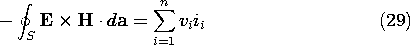
Figure 11.3.1 Distribution of Poynting flux in coaxial resistors and associated free space. The configuration is the same as for Example 7.5.2. A source to the left supplies current to disk-shaped and circular cylindrical resistive materials. The outer and right-end conductors are perfectly conducting. Note that there is a Poynting flux in the free space interior region even when the currents are stationary.

This distribution of S is sketched in Fig. 11.3.1. Wherever there is a dissipation density, there must be a negative divergence of S. Thus, in the conductors, the S lines terminate in the volume. In the free space region (a), S is solenoidal. Even with the fields perfectly stationary in time, the power is seen to flow through the open space to be absorbed in the volume where the dissipation takes place. The integral of the Poynting vector over the surface surrounding the inner conductor gives what we would expect either from the circuit point of view

where i is the total current through the cylinder, or from an evaluation of the right-hand side of the integral conservation law.

An Alternative Conservation Theorem for Electroquasistatic Systems

In describing electroquasistatic systems, it is inconvenient to require that the magnetic field intensity be evaluated. We consider now an alternative conservation theorem that is specialized to EQS systems. We will find an alternative expression for S that does not involve H. In the process of finding an alternative distribution of S, we illustrate the danger of ascribing meaning to S evaluated at a point, rather than integrated over a closed surface.

In the EQS approximation, E is irrotational. Thus,

and the power input term on the left in the integral conservation law, (11.1.1), can be expressed as

Next, the vector identity

is used to write the right-hand side of (19) as

The first integral on the right is zero because the curl of a vector is divergence free and a field with no divergence has zero flux through a closed surface. Ampère's law can be used to eliminate curl H from the second.

In this way, we have determined an alternative expression for S, valid only in the electroquasistatic approximation.

The density of power flow, expressed by (23) as the product of a potential and total current density consisting of the sum of the conduction and displacement current densities, has a form similar to that used in circuit theory.

The power flux density of (23) is convenient in describing EQS systems, where the effects of magnetic induction are not significant. To be consistent with the EQS approximation, the conservation law must be used with the magnetic energy density neglected.

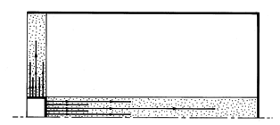
Example 11.3.2. Alternative EQS Power Flux Density for Stationary Current Distribution

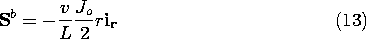
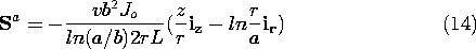
To contrast the alternative EQS power flow density with the Poynting flux density, consider again the coaxial resistor configuration of Example 11.3.1. Because the fields are stationary, the EQS power flux density is

By contrast with the Poynting flux density, this vector field is zero in the free space region. In the circular cylindrical conductor, the potential and current density are [(7.5.6) and (7.5.7)]

and it follows that the power flux density is simply

There is a similar, radially directed flux density in the disk-shaped resistor.

The alternative distribution of S, shown in Fig. 11.3.2, is clearly very different from that shown in Fig. 11.3.1 for the Poynting flux density.

Figure 11.3.2 Distribution of electroquasistatic flux density for the same system as shown in Fig. 11.3.1.

Poynting Power Density Related to Circuit Power Input

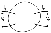
Suppose that the surface S described by the conservation theorem encloses a system that is accessed through terminal pairs, as shown in Fig. 11.3.3. Under what circumstances is the integral of S da over S equivalent to summing the voltage-current product of the terminals of the wires connected to the system?

Figure 11.3.3 Arbitrary EQS system accessed through terminal pairs.

Two attributes of the fields on the surface S enclosing the system are required. First, the contribution of the magnetic induction to E must be negligible on S. If this is so, then regardless of what is inside S (for example, both EQS and MQS systems), on the surface S, the electric field can be taken as irrotational. It follows that in taking the integral over a closed surface of the Poynting power density, we can just as well use (23).

By contrast with the EQS systems treated in deriving this expression, it now holds only on the surface S, not necessarily on surfaces inside the volume enclosed by S.

Second, on the surface S, the contribution of the displacement current must be negligible. This is equivalent to requiring that S is chosen parallel to the displacement flux density. In this case, the total power into the system reduces to

The integrand has value only where the surface S intersects a wire. If taken as perfectly conducting (but nevertheless in a region where B/ t is zero and hence E is irrotational), the wires have potentials that are uniform over their cross-sections. Thus, in (28), is equal to the voltage of the terminal. In integrating the current density over the cross-section of the wire, note that da is directed out of the surface, while a positive terminal current is directed into the surface. Thus,

and the input power expressed by (28) is equivalent to what would be expected from circuit theory.

Poynting Flux and Electromagnetic Radiation

Power cannot be supplied to or lost by a quasistatic system of finite extent through a surface at infinity. Such a power supply or loss requires radiation, and electromagnetic waves are neglected when either the magnetic induction or the displacement current density are neglected. To prove this statement, consider an EQS system of finite net charge. Its electric field intensity decays like 1/r² at infinity, where r is the distance to a far-off point from some origin chosen within the system. At a great distance, the currents appear equivalent to current loop sources. Hence, the magnetic field intensity has the 1/r³ decay typical of a magnetic dipole. It follows that the Poynting vector decays at least as fast as 1/r⁵, so that the flux of E x H integrated over the "sphere" at infinity of area 4 r² gives zero contribution. Because it is only that part of E x H resulting from electromagnetic radiation that contributes at infinity, Poynting's theorem is shown in Sec. 12.5 to be a powerful tool for dealing with antennae.