12.5
Complex Poynting's Theorem and Radiation Resistance

To the generator supplying its terminal current, a radiating antenna appears as a load with an impedance having a resistive part. This is true even if the antenna is made from perfectly conducting material and therefore incapable of converting electrical power to heat. The power radiated away from the antenna must be supplied through its terminals, much as if it were dissipated in a resistor. Indeed, if there is no electrical dissipation in the antenna, the power supplied at the terminals is that radiated away. This statement of power conservation makes it possible to determine the equivalent resistance of the antenna simply by using the far fields that were the theme of Sec. 12.4.

Complex Poynting's Theorem

For systems in the sinusoidal steady state, a useful alternative to the form of Poynting's theorem introduced in Secs. 11.1 and 11.2 results from writing Maxwell's equations in terms of complex amplitudes before they are combined to provide the desired theorem. That is, we assume at the outset that fields and sources take the form

Suppose that the region of interest is composed either of free space or of perfect conductors. Then, substitution of complex amplitudes into the laws of Ampère and Faraday, (12.0.8) and (12.0.9), gives

The manipulations that are now used to obtain the desired "complex Poynting's theorem" parallel those used to derive the real, time-dependent form of Poynting's theorem in Sec. 11.2. We dot E with the complex conjugate of (2) and subtract the dot product of the complex conjugate of H with (3). It follows that ⁸

The object of this manipulation was to obtain the "perfect" divergence on the left, because this expression can then be integrated over a volume V and Gauss' theorem used to convert the volume integral on the left to an integral over the enclosing surface S.

⁸ (A x B) = B x A - A x B

This expression has been multiplied by , so that its real part represents the time average flow of power, familiar from Sec. 11.5. Note that the real part of the first term on the right is zero. The real part of (5) equates the time average of the Poynting vector flux into the volume with the time average of the power imparted to the current density of unpaired charge, J_u, by the electric field. This information is equivalent to the time average of the (real form of) Poynting's theorem. The imaginary part of (5) relates the difference between the time average magnetic and electric energies in the volume V to the imaginary part of the complex Poynting flux into the volume. The imaginary part of the complex Poynting theorem conveys additional information.

Radiation Resistance

Consider the perfectly conducting antenna system surrounded by the spherical surface, S, shown in Fig. 12.5.1. To exclude sources from the enclosed volume, this surface is composed of an outer surface, S_a, that is far enough from the antenna so that only the radiation field makes a contribution, a surface S_b that surrounds the source(s), and a surface S_c that can be envisioned as the wall of a system of thin tubes connecting S_a to S_b in such a way that S_a + S_b + S_c is indeed the surface enclosing V. By making the connecting tubes very thin, contributions to the integral on the left in (5) from the surface S_c are negligible. We now write, and then explain, the terms in (5) as they describe this radiation system.

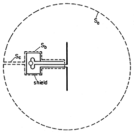
The first term is the contribution from integrating the radiation Poynting flux over S_a, where (12.4.2) serves to eliminate H. The second term comes from the surface integral in (5) of the Poynting flux over the surface, S_b, enclosing the sources (generators). Think of the generators as enclosed by perfectly conducting boxes powered by terminal pairs (coaxial cables) to which the antennae are attached. We have shown in Sec. 11.3 (11.3.29) that the integral of the Poynting flux over S_b is equivalent to the sum of voltage-current products expressing power flow from the circuit point of view. The first term on the right is the same as the first on the right in (5). Finally, the last term in (5) makes no contribution, because the only regions where J exists within V are those modeled here as perfectly conducting and hence where E = 0.

Consider a single antenna with one input terminal pair. The antenna is a linear system, so the complex voltage must be proportional to the complex terminal current.

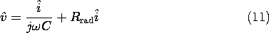
Here, Z_ant is the impedance of the antenna. In terms of this impedance, the time average power can be written as

It follows from the real part of (6) that the radiation resistance, R_rad, is

The imaginary part of Z_out describes the reactive power supplied to the antenna.

The radiation field contributions to this integral cancel out. If the antenna elements are short compared to a wavelength, contributions to (10) are dominated by the quasistatic fields. Thus, the electric dipole contributions are dominated by the electric field (and the reactance is capacitive), while those for the magnetic dipole are inductive. By making the antenna on the order of a wavelength, the magnetic and electric contributions to (10) are often made to essentially cancel. An example is a half-wavelength version of the wire antenna in Example 12.4.1. The equivalent circuit for such resonant antennae is then solely the radiation resistance.

Example 12.5.1. Equivalent Circuit of an Electric Dipole

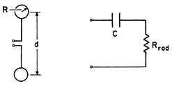
An "end-loaded" electric dipole is composed of a pair of perfectly conducting metal spheres, each of radius R, as shown in Fig. 12.5.2. These spheres have a spacing, d, that is short compared to a wavelength but large compared to the radius, R, of the spheres.

Figure 12.5.2 End-loaded dipole and equivalent circuit.

The equivalent circuit is also shown in Fig. 12.5.2. The statement that the sum of the voltage drops around the circuit is zero requires that

A statement of power flow is obtained by multiplying this expression by the complex conjugate of the complex amplitude of the current.

Here the dipole charge, q, is defined such that i = dq/dt. The real part of this expression takes the same form as the statement of complex power flow for the antenna, (6). Thus, with provided by (12.2.23) and (12.2.24), we can solve for the radiation resistance:

Note that because k /c, this radiation resistance is proportional to the square of the frequency.

The imaginary part of the impedance is given by the right-hand side of (10). The radiation field contributions to this integral cancel out. In integrating over the near field, the electric energy storage dominates and becomes essentially that associated with the quasistatic capacitance of the pair of spheres. We assume that the spheres are connected by wires that are extremely thin, so that their effect can be ignored. Then, the capacitance is the series capacitance of two isolated spheres, each having a capacitance of 4 R.

Radiation fields are solutions to the full Maxwell equations. In contrast, EQS fields were analyzed ignoring the magnetic flux linkage in Faraday's law. The approximation is justified if the size of the system is small compared with a wavelength. The following example treats the scattering of particles that are small compared with the wavelength. The fields around the particles are EQS, and the currents induced in the particles are deduced from the EQS approximation. These currents drive radiation fields, resulting in Rayleigh scattering. The theory of Rayleigh scattering explains why the sky is blue in color, as the following example shows.

Example 12.5.2. Rayleigh Scattering

Consider a spatial distribution of particles in the field of an infinite parallel plane wave. The particles are assumed to be small as compared to the wavelength of the plane wave. They get polarized in the presence of an electric field E_a, acquiring a dipole moment

where is the polarizability. These particles could be atoms or molecules, such as the molecules of nitrogen and oxygen of air exposed to visible light. They could also be conducting spheres of radius R. In the latter case, the dipole moment produced by an applied electric field E_a is given by (6.6.5) and the polarizability is

If the frequency of the polarizing wave is and its propagation constant k = /c, the far field radiated by the particle, expressed in a spherical coordinate system with its = 0 axis aligned with the electric field of the wave, is, from (12.2.22),

where d = j is used in the above expression. The power radiated by each dipole, i.e., the power scattered by a dipole, is

The scattered power increases with the fourth power of frequency when is not a function of frequency. The polarizability of N₂ and O₂ is roughly frequency independent. Of the visible radiation, the blue (high) frequencies scatter much more than the red (low) frequencies. This is the reason for the blue color of the sky. The same phenomenon accounts for the polarization of the scattered radiation. Along a line L at a large angle from the line from the observer O to the sun S, only the electric field perpendicular to the plane LOS produces radiation visible at the observer position (note the sin² dependence of the radiation). Thus, the scattered radiation observed at O has an electric field perpendicular to LOS.

The present analysis has made two approximations. First, of course, we assumed that the particle is small compared with a wavelength. Second, we computed the induced polarization from the unperturbed field E of the incident plane wave. This assumes that the particle perturbs the wave negligibly, that the scattered power is very small compared to the power in the wave. Of course, the incident wave decreases in intensity as it proceeds through the distribution of scatterers, but this macroscopic change can be treated as a simple attenuation proportional to the density of scatterers.