13.2
Two-Dimensional Modes Between Parallel Plates
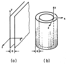
This section treats the boundary value approach to finding the fields between the perfectly conducting parallel plates shown in Fig. 13.2.1a. Most of the mathematical ideas and physical insights that come from a study of modes on perfectly conducting structures that are uniform in one direction (for example, parallel wire and coaxial transmission lines and waveguides in the form of hollow perfectly conducting tubes) are illustrated by this example. In the previous section, we have already seen that the plates can be used as a transmission line supporting TEM waves. In this and the next section, we shall see that they are capable of supporting other electromagnetic waves.
Figure 13.2.1 (a) Plane parallel perfectly conducting plates. (b) Coaxial geometry in which z-independent fields of (a) might be approximately obtained without edge effects. Because the structure is uniform in the z direction, it can be excited in such a way that fields are independent of z. One way to make the structure approximately uniform in the z direction is illustrated in Fig. 13.2.1b, where the region between the plates becomes the annulus of coaxial conductors having very nearly the same radii. Thus, the difference of these radii becomes essentially the spacing a and the z coordinate maps into the
coordinate. Another way is to make the plates very wide (in the z direction) compared to their spacing, a. Then, the fringing fields from the edges of the plates are negligible. In either case, the understanding is that the field excitation is uniformly distributed in the z direction. The fields are now assumed to be independent of z.
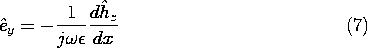
Because the fields are two dimensional, the classifications and relations given in Sec. 12.6 and summarized in Table 12.8.3 serve as our starting point. Cartesian coordinates are appropriate because the plates lie in coordinate planes. Fields either have H transverse to the x - y plane and E in the x - y plane (TM) or have E transverse and H in the x - y plane (TE). In these cases, Hz and Ez are taken as the functions from which all other field components can be derived. We consider sinusoidal steady state solutions, so these fields take the form
These field components, respectively, satisfy the Helmholtz equation, (12.6.9) and (12.6.33) in Table 12.8.3, and the associated fields are given in terms of these components by the remaining relations in that table.
Once again, we find product solutions to the Helmholtz equation, where Hz and Ez are assumed to take the form X(x) Y(y). This formalism for reducing a partial differential equation to ordinary differential equations was illustrated for Helmholtz's equation in Sec. 12.6. This time, we take a more mature approach, based on the observation that the coefficients of the governing equation are independent of y (are constants). As a result, Y(y) will turn out to be governed by a constant coefficient differential equation. This equation will have exponential solutions. Thus, with the understanding that ky is a yet to be determined constant (that will turn out to have two values), we assume that the solutions take the specific product forms
Then, the field relations of Table 12.8.3 become
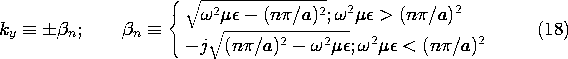
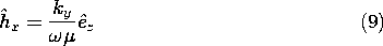
TM Fields:
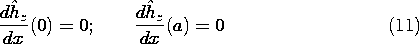
where p2

2
- ky2
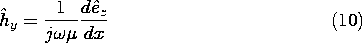
TE Fields:
where q2
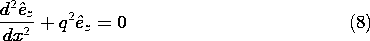
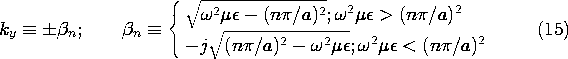
The boundary value problem now takes a classic form familiar from Sec. 5.5. What values of p and q will make the electric field tangential to the plates zero? For the TM fields,
y = 0 on the plates, and it follows from (7) that it is the derivative of Hz that must be zero on the plates. For the TE fields, Ez must itself be zero at the plates. Thus, the boundary conditions are
TM Fields:
TE Fields:
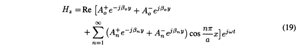
To check that all of the conditions are indeed met at the boundaries, note that if (11) is satisfied, there is neither a tangential E nor a normal H at the boundaries for the TM fields. (There is no normal H whether the boundary condition is satisfied or not.) For the TE field, Ez is the only electric field, and making Ez=0 on the boundaries indeed guarantees that Hx = 0 there, as can be seen from (9).
Representing the TM modes, the solution to (5) is a linear combination of sin (px) and cos (px). To satisfy the boundary condition, (11), at x = 0, we must select cos (px). Then, to satisfy the condition at x = a, it follows that p = pn = n
/a, n = 0, 1, 2,

Dependence of fundamental fields on $x$.
These functions and the associated values of p are called eigenfunctions and eigenvalues, respectively. The solutions that have been found have the x dependence shown in Fig. 13.2.2a.
Figure 13.2.2 Dependence of fundamental fields on x. From the definition of p given in (5), it follows that for a given frequency
Similar reasoning identifies the modes for the TE fields. Of the two solutions to (8), the one that satisfies the boundary condition at x = 0 is sin (qx). The second boundary condition then requires that q take on certain eigenvalues, qn.
The x dependence of Ez is then as shown in Fig. 13.2.2b. Note that the case n = 0 is excluded because it implies a solution of zero amplitude.
For the TE fields, it follows from (17) and the definition of q given with (8) that


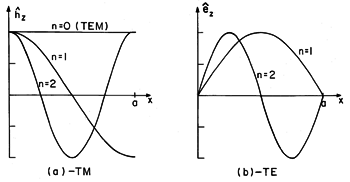


5 For the particular geometry considered here, it has turned out that the eigenvalues pn and qn are the same (with the exception of n = 0). This coincidence does not occur with boundaries having other geometries.
In general, the fields between the plates are a linear combination of all of the modes. In superimposing these modes, we recognize that ky =

n. Thus, with coefficients that will be determined by boundary conditions in planes of constant y, we have the solutions
TM Modes:
TE Modes:
We shall refer to the n-th mode represented by these fields as the TMn or TEn mode, respectively.
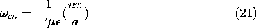
We now make an observation about the TM0 mode that is of far-reaching significance. Its distribution of Hz has no dependence on x [(13) with pn = 0]. As a result, Ey = 0 according to (7). Thus, for the TM0 mode, both E and H are transverse to the axial direction y. This special mode, represented by the n = 0 terms in (19), is therefore the transverse electromagnetic (TEM) mode featured in the previous section. One of its most significant features is that the relation between frequency
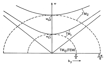
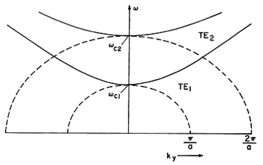
The frequency dependence of ky for the TEM mode and for the higher-order TMn modes given by (15) are represented graphically by the
Figure 13.2.3 Dispersion relation for TM modes. The velocity of propagation of points of constant phase (for example, a point at which a field component is zero) is
The dispersion equation for the TE modes is shown in Fig. 13.2.4. Although the field distributions implied by each branch are very different, in the case of the plane parallel electrodes considered here, the curves are the same as those for the TMn
0 modes.
Figure 13. Dispersion relation for TE modes. The next section will provide greater insight into the higher-order TM and TE modes.