13.4
Rectangular Waveguide Modes

Metal pipe waveguides are often used to guide electromagnetic waves. The most common waveguides have rectangular cross-sections and so are well suited for the exploration of electrodynamic fields that depend on three dimensions. Although we confine ourselves to a rectangular cross-section and hence Cartesian coordinates, the classification of waveguide modes and the general approach used here are equally applicable to other geometries, for example to waveguides of circular cross-section.

The parallel plate system considered in the previous three sections illustrates much of what can be expected in pipe waveguides. However, unlike the parallel plates, which can support TEM modes as well as higher-order TE modes and TM modes, the pipe cannot transmit a TEM mode. From the parallel plate system, we expect that a waveguide will support propagating modes only if the frequency is high enough to make the greater interior cross-sectional dimension of the pipe greater than a free space half-wavelength. Thus, we will find that a guide having a larger dimension greater than 5 cm would typically be used to guide energy having a frequency of 3 GHz.

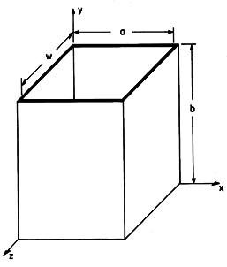
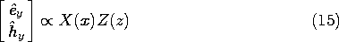
Figure 13.4.1 Rectangular waveguide.

We found it convenient to classify two-dimensional fields as transverse magnetic (TM) or transverse electric (TE) according to whether E or H was transverse to the direction of propagation (or decay). Here, where we deal with three-dimensional fields, it will be convenient to classify fields according to whether they have E or H transverse to the axial direction of the guide. This classification is used regardless of the cross-sectional geometry of the pipe. We choose again the y coordinate as the axis of the guide, as shown in Fig. 13.4.1. If we focus on solutions to Maxwell's equations taking the form

then all of the other complex amplitude field components can be written in terms of the complex amplitudes of these axial fields, H_y and E_y. This can be seen from substituting fields having the form of (1) and (2) into the transverse components of Ampère's law, (12.0.8),

and into the transverse components of Faraday's law, (12.0.9),

If we take _y and _y as specified, (3) and (6) constitute two algebraic equations in the unknowns _x and _z. Thus, they can be solved for these components. Similarly, _x and _z follow from (4) and (5).

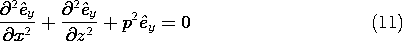
We have found that the three-dimensional fields are a superposition of those associated with E_y (so that the magnetic field is transverse to the guide axis ), the TM fields, and those due to H_y, the TE modes. The axial field components now play the role of "potentials" from which the other field components can be derived.

We can use the y components of the laws of Ampère and Faraday together with Gauss' law and the divergence law for H to show that the axial complex amplitudes _y and _y satisfy the two-dimensional Helmholtz equations.

TM Modes (H_y = 0):

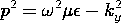
where

and

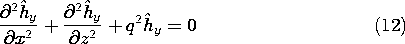
TE Modes (E_y = 0):

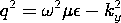
where

These relations also follow from substitution of (1) and (2) into the y components of (13.0.2) and (13.0.1).

The solutions to (11) and (12) must satisfy boundary conditions on the perfectly conducting walls. Because E_y is parallel to the perfectly conducting walls, it must be zero there.

TM Modes:

The boundary condition on H_y follows from (9) and (10), which express _x and _z in terms of _y. On the walls at x = 0 and x = a, _z = 0. On the walls at z = 0, z = w, _x = 0. Therefore, from (9) and (10) we obtain

TE Modes:

The derivative of _y with respect to a coordinate perpendicular to the boundary must be zero.

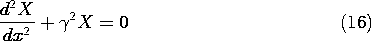
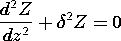
The solution to the Helmholtz equation, (11) or (12), follows a pattern that is familiar from that used for Laplace's equation in Sec. 5.4. Either of the complex amplitudes representing the axial fields is represented by a product solution.

Substitution into (11) or (12) and separation of variables then gives

where

Solutions that satisfy the TM boundary conditions, (13), are then

TM Modes:

so that

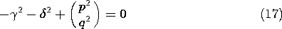
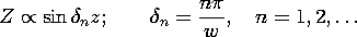
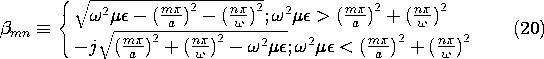
When either m or n is zero, the field is zero, and thus m and n must be equal to an integer equal to or greater than one. For a given frequency and mode number (m, n), the wave number k_y is found by using (19) in the definition of p associated with (11)

with

Thus, the TM solutions are

For the TE modes, (14) provides the boundary conditions, and we are led to the solutions

TE Modes:

Substitution of _m and _n into (17) therefore gives

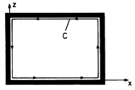
The wave number k_y is obtained using this eigenvalue in the definition of q associated with (12). With the understanding that either m or n can now be zero, the expression is the same as that for the TM modes, (20). However, both m and n cannot be zero. If they were, it follows from (22) that the axial H would be uniform over any given cross-section of the guide. The integral of Faraday's law over the cross-section of the guide, with the enclosing contour C adjacent to the perfectly conducting boundaries as shown in Fig. 13.4.2, requires that

where A is the cross-sectional area of the guide. Because the contour on the left is adjacent to the perfectly conducting boundaries, the line integral of E must be zero. It follows that for the m = 0, n = 0 mode, H_y = 0. If there were such a mode, it would have both E and H transverse to the guide axis. We will show in Sec. 14.2, where TEM modes are considered in general, that TEM modes cannot exist within a perfectly conducting pipe.

Figure 13.4.2 Cross-section of guide with contour adjacent to perfectly conducting walls.

Even though the dispersion equations for the TM and TE modes only differ in the allowed lowest values of (m, n), the field distributions of these modes are very different.

---

⁹ In other geometries, such as a circular waveguide, this coincidence of p_mn and q_mn is not found.

---

The superposition of TE modes gives

where m n 0. The frequency at which a given mode switches from evanescence to propagation is an important parameter. This cutoff frequency follows from (20) as

TM Modes:

TE Modes:

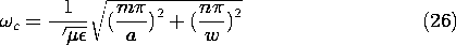
Rearranging this expression gives the normalized cutoff frequency as functions of the aspect ratio a/w of the guide.

These normalized cutoff frequencies are shown as functions of w/a in Fig. 13.4.3.

Figure 13.4.3 Normalized cutoff frequencies for lowest rectangular waveguide modes as a function of aspect ratio.

The numbering of the modes is standardized. The dimension w is chosen as w a, and the first index m gives the variation of the field along a. The TE₁₀ mode then has the lowest cutoff frequency and is called the dominant mode. All other modes have higher cutoff frequencies (except, of course, in the case of the square cross-section for which TE₀₁ has the same cutoff frequency). Guides are usually designed so that at the frequency of operation only the dominant mode is propagating, while all higher-order modes are "cutoff."

In general, an excitation of the guide at a cross-section y = constant excites all waveguide modes. The modes with cutoff frequencies higher than the frequency of excitation decay away from the source. Only the dominant mode has a sinusoidal dependence upon y and thus possesses fields that are periodic in y and "dominate" the field pattern far away from the source, at distances larger than the transverse dimensions of the waveguide.

Example 13.4.1. TE₁₀ Standing Wave Fields

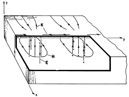
The section of rectangular guide shown in Fig. 13.4.4 is excited somewhere to the right of y = 0 and shorted by a conducting plate in the plane y = 0. We presume that the frequency is above the cutoff frequency for the TE₁₀ mode and that a > w as shown. The frequency of excitation is chosen to be below the cutoff frequency for all higher order modes and the source is far away from y = 0 (i.e., at y a). The field in the guide is then that of the TE₁₀ mode. Thus, H_y is given by (25) with m = 1 and n = 0. What is the space-time dependence of the standing waves that result from having shorted the guide?

Figure 13.4.4 Fields and surface sources for TE₁₀ mode.

Because of the short, E_z (x, y = 0, z) = 0. In order to relate the coefficients C⁺₁₀ and C^-₁₀, we must determine _z from _y as given by (25) using (10)

and because _z = 0 at the short, it follows that

so that

and this is the only component of the electric field in this mode. We can now use (29) to evaluate (25).

In using (7) to evaluate the other component of H, remember that in the C⁺_mn term of (25), k_y = _mn, while in the C^-_mn term, k_y = -_mn.

To sketch these fields in the neighborhood of the short and deduce the associated surface charge and current densities, consider C⁺₁₀ to be real. The j in (31) and (32) shows that H_x and H_y are 90 degrees out of phase with the electric field. Thus, in the field sketches of Fig. 13.4.4, E and H are shown at different instants of time, say E when t = and H when t = /2. The surface charge density is where E_z terminates and originates on the upper and lower walls. The surface current density can be inferred from Ampère's continuity condition. The temporal oscillations of these fields should be pictured with H equal to zero when E peaks, and with E equal to zero when H peaks. At planes spaced by multiples of a half-wavelength along the y axis, E is always zero.

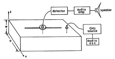
The following demonstration illustrates how a movable probe designed to couple to the electric field is introduced into a waveguide with minimal disturbance of the wall currents.

Demonstration 13.4.1. Probing the TE₁₀Mode.

A waveguide slotted line is shown in Fig. 13.4.5. Here the line is shorted at y = 0 and excited at the right. The probe used to excite the guide is of the capacitive type, positioned so that charges induced on its tip couple to the lines of electric field shown in Fig. 13.4.4. This electrical coupling is an alternative to the magnetic coupling used for the TE mode in Demonstration 13.3.2.

Figure 13.4.5 Slotted line for measuring axial distribution of TE₁₀ fields.

The y dependence of the field pattern is detected in the apparatus shown in Fig. 13.4.5 by means of a second capacitive electrode introduced through a slot so that it can be moved in the y direction and not perturb the field, i.e., the wall is cut along the lines of the surface current K. From the sketch of K given in Fig. 13.4.4, it can be seen that K is in the y direction along the center line of the guide.

The probe can be used to measure the wavelength 2 /k_y of the standing waves by measuring the distance between nulls in the output signal (between nulls in E_z). With the frequency somewhat below the cutoff of the TE₁₀ mode, the spatial decay away from the source of the evanescent wave also can be detected.