14.6
Reflection Coefficient Representation of Transmission Lines

In Sec. 14.5, we found that a quarter-wavelength of transmission line turned a short circuit into an open circuit. Indeed, with an appropriate length (or driven at an appropriate frequency), the shorted line could have an inductive or a capacitive reactance. In general, the impedance observed at the terminals of a transmission line has a more complicated dependence on the termination.

Typical microwave measurements are made with a length of transmission line between the observation point and the terminals of the device under study, whether that be an antenna or a transistor. In this section, the objective is a way of visualizing the relation between the impedance at the "generator" terminals and the impedance of the "load." We will find that a representation of the variables in the reflection coefficient plane is valuable both conceptually and practically.

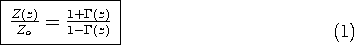
At a location z, the impedance of the transmission line shown in Fig. 14.6.1a is (14.5.10)

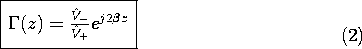
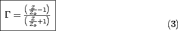
where the reflection coefficient at the location z is defined as the complex function

At the load position, where z = 0, the reflection coefficient is equal to _L as defined by (14.5.11).

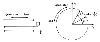
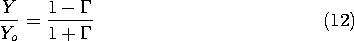
Fig 14.6.1 (a)Transmission line conventions. (b) Reflection coefficient dependence on z in the complex plane.

Like the impedance, the reflection coefficient is a function of z. Unlike the impedance, has an easily pictured z dependence. Regardless of z, the magnitude of is the same. Thus, as pictured in the complex plane of Fig. 14.6.1b, it is a complex vector of magnitude |_-/₊| and angle + 2 z, where is the angle at the position z = 0. With z defined as increasing from the generator to the load, the dependence of the reflection coefficient on z is as summarized in the figure. As we move from the generator toward the load, z increases and hence rotates in the counterclockwise direction.

In summary, once the complex number is established at one location z, its variation as we move toward the load or toward the generator can be pictured as a rotation at constant magnitude in the counterclockwise or clockwise directions, respectively. Typically, is established at the location of the load, where the impedance, Z_L, is known. Then at any location z follows from (1) solved for .

With the magnitude and phase of established at the load, the reflection coefficient can be found at another location by a simple rotation through an angle 4 (z/ ), as shown in Fig. 14.6.1b. The impedance at this second location would then follow from evaluation of (1).

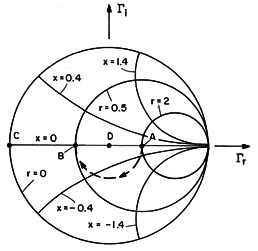
Smith Chart

We save ourselves the trouble of evaluating (1) or (3), either to establish at the load or to infer the impedance implied by at some other location, by mapping Z/Z_o in the plane of Fig. 14.6.1b. To this end, we define the normalized impedance as having a resistive part r and a reactive part x

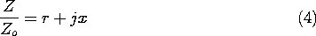
and plot the contours of constant r and of constant x in the plane. This makes it possible to see directly what Z is implied by each value of . Effectively, such a mapping provides a graphical solution of (1). The next few steps summarize how this mapping of the contours of constant r and x in the _r - _i plane can be made with ruler and compass.

First, (1) is written using (4) on the left and = _r + j_i on the right. The real and imaginary parts of this equation must be equal, so it follows that

These expressions are quadratic in _r and _i. By completing the squares, they can be written as

Thus, the contours of constant normalized resistance, r, and of constant normalized reactance, x, are the circles shown in Figs. 14.6.2a-14.6.2b.

Fig 14.6.2 (a) Circle of constant normalized resistance, r, in plane. (b) Circle of constant normalized reactance, x, in plane.

Putting these contours together gives the lines of constant r and x in the complex plane shown in Fig. 14.6.3. This is called a Smith chart.

Fig 14.6.3 Smith chart.

Illustration. Impedance with Simple Terminations

How do we interpret the examples of Sec. 14.5 in terms of the Smith chart?

Quarter-wave Section. In Example 14.5.3 we found that a normalized resistive load r_L was transformed into its reciprocal by a quarter-wave line. Suppose that r_L = 2 (the load resistance is 2Z_o) and x = 0. Then, the load is at A in Fig. 14.6.3. A quarter-wavelength toward the generator is a rotation of 180 degrees in a clockwise direction, with following the trajectory from A B in Fig. 14.6.3. Note that the impedance at B is indeed the reciprocal of that at A, r = 0.5, x = 0.

Impedance of Short Circuit Line. Consider next the shorted line of Example 14.5.2. The load resistance r_L is 0, and reactance x_L is 0 as well, so we begin at the point C in Fig. 14.6.3. Now, we can trace out the impedance as we move away from the short toward the generator by rotating along the trajectory of unit radius in the clockwise direction. Note that all along this trajectory, r = 0. The normalized reactance then traces out the values given in Fig. 14.5.2, first taking on positive (inductive) values until it becomes infinite at /4 (rotation of 180 degrees), and then negative (capacitive) values until it returns to C, when the line has a length of /2.

Matched Line. For the matched load of Example 14.5.1, we start out with r_L = 1 and x_L = 0. This is point D at the origin in Fig. 14.6.3. Thus, the trajectory of is a circle of zero radius, and the impedance remains r_L = 1 over the length of the line.

While taking measurements on a transmission line terminated in a particular device, the Smith chart is often used to have an immediate picture of the impedance at the terminals. Even though the chart could be replaced by a programmable calculator, the overview provided by the Smith chart is important. Not only does it provide insight concerning the impedance, it can be used to picture the spatial evolution of the voltage and current, as we now see.

Standing Wave Ratio

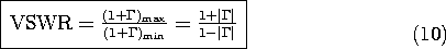
Once the reflection coefficient has been established, the voltage and current distributions are determined (to within a factor determined by the source). That is, in terms of , (14.5.5) becomes

The exponential factor has an amplitude that is independent of z. Thus, [1 + (z)] represents the z dependence of the voltage amplitude. This complex quantity can be pictured in the plane as shown in Fig. 14.6.4a. Remember, as we move from load to generator, rotates in the clockwise direction. As it does so, 1 + varies between a maximum value of 1 + | | and a minimum value of 1 - | |. According to (9), we can now picture the spatial distribution of the voltage amplitude. Convenient for describing this distribution is the voltage standing wave ratio (VSWR), defined as the ratio of the maximum voltage amplitude to the minimum voltage amplitude. From Fig. 14.6.4a, we can see that this ratio is

Fig 14.6.4 (a) Normalized line voltage 1 + . (b) Distribution of voltage amplitude for three VSWR's.

The distribution of voltage amplitude is shown for several VSWR's in Fig. 14.6.4b. We have already seen such distributions in two extremes. With the short circuit or open circuit terminations considered in Sec. 13.1, the reflection coefficient was on the unit circle and the VSWR was infinite. Indeed, the infinite VSWR envelope of Fig. 14.6.4b is that of a standing wave, with nulls every half-wavelength. The opposite extreme is also familiar. Here, the line is matched and the reflection coefficient is on a circle of zero radius. Thus, the VSWR is unity and the distribution of voltage amplitude is uniform.

Measurement of the VSWR and the location of a voltage null provides the information needed to determine a line termination. This follows by first using (10) to evaluate the magnitude of the reflection coefficient from the measured VSWR.

Thus, the radius of the circle representing the voltage distribution on the line has been determined. Second, a determination of the position of a null is tantamount to locating (to within a half-wavelength) the position on the line where passes through the negative real axis. The distance from this point to the load, in wavelengths, then determines where the load is located on this circle. The corresponding impedance is that of the load.

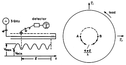
Demonstration 14.6.1. VSWR and Load Impedance

In the slotted line shown in Fig. 14.6.5, a movable probe with its attached detector provides a measure of the line voltage as a function of z. The distance between the load and the voltage probe can be measured directly. By using a frequency of 3 GHz and an air-insulated cable (having a permittivity that is essentially that of free space, so that the wave velocity is 3 x 10⁸ m/s), the wavelength is conveniently 10 cm.

Fig 14.6.5 Demonstration of distribution of voltage magnitude as function of VSWR.

The characteristic impedance of the coaxial cable is 50 , so with terminations of 50 , 100 , and a short, the observed distribution of voltage is as shown in Fig. 14.6.4b for VSWR's of 1, 2, and . (To plot data points on these curves, the measured values should be normalized to match the peak voltage of the appropriate distribution.)

Figure 14.6.5 illustrates how a measurement of the VSWR and position of a null can be used to infer the termination. Addition of a half-wavelength to l means an additional revolution in the plane, so which null is used to define the distance l makes no difference. The trajectory drawn in the illustration is for the 100 termination.

Admittance in the Reflection Coefficient Plane

Commonly, transmission lines are interconnected in parallel. It is then convenient to work with the admittance rather than the impedance. The Smith chart describes equally well the evolution of the admittance with z.

With Y_o = 1/Z_o defined as the characteristic admittance, it follows from (1) that

If -, this expression becomes identical to that relating the normalized impedance to , (1). Thus, the contours of constant normalized conductance, g, and normalized susceptance, y,

are those of the normalized impedance, r and x, rotated by 180 degrees. Rotate by 180 degrees the impedance form of the Smith chart and the admittance form is obtained! The contours of r and x, respectively, become those of g and y.

⁹ Usually, is not explicitly evaluated. Rather, the admittance is given at one point on the circle (and hence on the chart) and determined (by a rotation through the appropriate angle on the chart) at another point. Thus, for most applications, the chart need not even be rotated. However, if is to be evaluated directly from the admittance, it should be remembered that the coordinates are actually -_r and -_i.

The admittance form of the Smith chart is used in the following example.

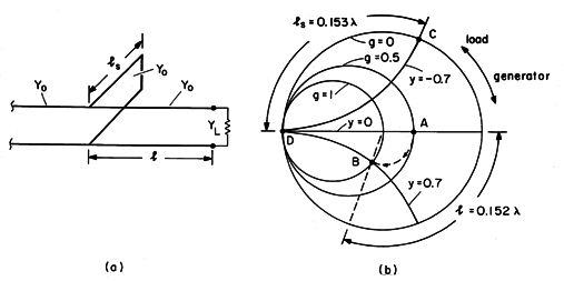
Example 14.6.1. Single Stub Matching

In Fig. 14.6.6a, the load admittance Y_L is to be matched to a transmission line having characteristic admittance Y_o by means of a "stub" consisting of a shorted section of line having the same characteristic admittance Y_o. Variables that can be used to accomplish the matching are the distance l from the load to the stub and the length l_s of the stub.

Fig 14.6.6 (a) Single stub matching. (b) Admittance Smith chart

Matching is accomplished in two steps. First, the length l is adjusted so that the real part of the admittance at the position where the stub is attached is equal to Y_o. Then the length of the shorted stub is adjusted so that it's susceptance cancels that of the line. Here, we see the reason for using the admittance form of the Smith chart, shown in Fig. 14.6.6b. The stub and the line are connected in parallel so that their admittances add.

The two steps are pictured in Fig. 14.6.6b for the case where the normalized load admittance is g + jy = 0.5, at A on the chart. The real part of the admittance becomes equal to the characteristic admittance on the circle g = 1; we adjust the length l so that the stub is connected at B, where the | | constant curve intersects the g = 1 circle. In the particular example shown, this length is l = 0.152 . From the chart, one reads off a positive susceptibility at this point of about y = 0.7. We can determine the stub length l_s that gives the negative of this susceptance by again using the chart. The desired admittance of the stub is at C, where g = 0 and y = -0.7. In the case of the stub, the "load" is the short, where the admittance is infinite, at D on the chart. Following the | | = 1 circle in the clockwise direction (from the "load" toward the "generator") from the short at D to the desired admittance at C then gives the length of the stub. For the example, l_s = 0.153 .

To the left of the point where the stub is attached, the line should have a unity VSWR. The following demonstrates this concept.

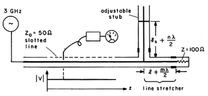
Demonstration 14.6.2. Single Stub Matching

In Fig. 14.6.7, the previous demonstration has been terminated with an adjustable length of line (a line stretcher) and a stub. The slotted line makes it possible to see the effect on the VSWR of matching the line. With a load of Z = 100 and the stub and line stretcher adjusted to the values found in the previous example, the voltage amplitude is found to be independent of the position of the probe in the slotted line. Of course, we can add a half-wavelength to either l or l_s and obtain the same condition.

Fig 14.6.7 Single stub matching demonstration.