Distributed Parameter Equivalents and Models | |||||||||
|---|---|---|---|---|---|---|---|---|---|
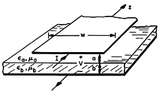
| 14.1.1 | The "strip line" shown in Fig. P14.1.1 is an example where the fields
are not exactly TEM. Nevertheless, wavelengths long
compared to a and b, the distributed parameter model is
applicable. The lower perfectly conducting plate is covered by a
planar perfectly insulating layer having properties ( b, b,  b =
o). Between this layer and the upper electrode is a second
perfectly insulating material having properties (a, a =
o). The width w is much greater than a + b, so fringing
fields can be ignored. Determine L and C and hence the
transmission line equations. Show that LC b =
o). Between this layer and the upper electrode is a second
perfectly insulating material having properties (a, a =
o). The width w is much greater than a + b, so fringing
fields can be ignored. Determine L and C and hence the
transmission line equations. Show that LC  unless a
= b. unless a
= b.
 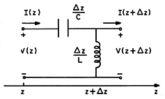 | ||||||||
| 14.1.2 | An incremental section of a "backward wave" transmission line is as
shown in Fig. P14.1.2. The incremental section of length  z
shown has a reciprocal capacitance per unit length z C-1 and
reciprocal inductance per unit length z L-1. Show that, by
contrast with (4) and (5), in this case the
transmission line equations are z
shown has a reciprocal capacitance per unit length z C-1 and
reciprocal inductance per unit length z L-1. Show that, by
contrast with (4) and (5), in this case the
transmission line equations are
 | ||||||||
Transverse Electromagnetic Waves | |||||||||
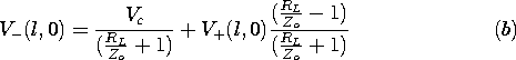
| 14.2.1* | For the coaxial configuration of Fig. 14.2.2b,
and  are are
  l is the charge per unit length on the inner
conductor. l is the charge per unit length on the inner
conductor.
| ||||||||
| 14.2.2 | A transmission line consists of a conductor having the cross-section shown in Fig. P4.7.5 adjacent to an L-shaped return conductor comprised of "ground planes" in the planes x = 0 and y = 0, intersecting at the origin. Assuming that the region between these conductors is free space, what are the transmission line parameters L and C? | ||||||||
Transients on Infinite Transmission Lines | |||||||||
| 14.3.1 | Show that the characteristic impedance of a coaxial cable (Prob.
14.2.1) is
 = 2.5 o and = o, evaluate
Zo for values of a/b = 2, 10, 100, and 1000. Would it be
reasonable to design such a cable to have Zo = 1 K = 2.5 o and = o, evaluate
Zo for values of a/b = 2, 10, 100, and 1000. Would it be
reasonable to design such a cable to have Zo = 1 K ? ?
| ||||||||
| 14.3.2 | For the parallel conductor line of Fig. 14.2.2 in free space, what value of l/R should be used to make Zo = 300 ohms? | ||||||||
| 14.3.3 | The initial conditions on an infinite line are V = 0 and I = Ip
for -d < z < d and I = 0 for z < -d and d < z. Determine
V(z, t) and I(z, t) for 0 < t, presenting the solution
graphically, as in Fig. 14.3.2.
| ||||||||
| 14.3.4 | On an infinite line, when t = 0, V = Vo exp (-z2/2a2), and I
= 0, determine analytical expressions for V(z, t) and I(z, t).
| ||||||||
| 14.3.5* | In the energy conservation theorem for a transmission line, (14.2.19),
VI is the power flow. Show that at any location, z, and time,
t, it is correct to think of power flow as the superposition of
power carried by the + wave in the +z direction and - wave in
the -z direction.
 | ||||||||
| 14.3.6 | Show that the traveling wave solutions of (2) are not solutions of
the equations for the "backward wave" transmission line of
Prob. 14.1.2.
| ||||||||
Transients on Bounded Transmission Lines | |||||||||
| 14.4.1 | A transmission line, terminated at z = l in an "open circuit," is
driven at z = 0 by a voltage source Vg in series with a
resistor, Rg, that is matched to the characteristic impedance of
the line, Rg = Zo. For t < 0, Vg = Vo = constant. For 0
< t, Vg = 0. Determine the distribution of voltage and current
on the line for 0 < t.
| ||||||||
| 14.4.2 | The transient is to be determined as in Prob. 14.4.1, except the line is now terminated at z = l in a "short circuit." | ||||||||
| 14.4.3 | The transmission line of Fig. 14.4.1 is terminated in a resistance
RL = Zo. Show that, provided that the voltage and current
over the length of the line are initially zero, the line has the same
effect on the circuit connected at z = 0 as would a resistance
Zo.
| ||||||||
| 14.4.4 | A transmission line having characteristic impedance Za is
terminated at z = l + L in a resistance Ra = Za. At the other
end, where z = l, it is connected to a second transmission line
having the characteristic impedance Zb. This line is driven at z
= 0 by a voltage source Vg(t) in series with a resistance Rb =
Zb. With Vg = 0 for t < 0, the driving voltage makes a step
change to Vg = Vo, a constant voltage. Determine the voltage
V(0, t).
| ||||||||
| 14.4.5 | A pair of transmission lines is connected as in Prob. 14.4.4.
However, rather than being turned on when t = 0, the voltage source
has been on for a long time and when t = 0 is suddenly turned off.
Thus, Vg = Vo for t < 0 and Vg = 0 for 0 < t. The lines
have the same wave velocity c. Determine V(0, t). (Note that,
by contrast with the situation in Prob. 14.4.4, the line having
characteristic impedance Za now has initial values of voltage and
current.)
| ||||||||
| 14.4.6 | A transmission line is terminated at z = l in a "short" and
driven at z = 0 by a current source Ig(t) in parallel with a
resistance Rg. For 0 < t < T, Ig = Io = constant, while for
t < 0 and T < t, Ig = 0. For Rg = Zo, determine V(0,
t).
| ||||||||
| 14.4.7 | With Rg not necessarily equal to Zo, the line of Prob. 14.4.6
is driven by a step in current; for t < 0, Ig = 0, while for 0
< t, Ig = Io = constant.
the current I(0, t).
| ||||||||
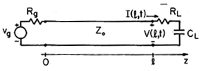
| 14.4.8 | The transmission line shown in Fig. P14.4.8 is terminated in a series
load resistance, RL, and capacitance CL.
reflected wave at z = l, given by (8) for the load resistance alone, is replaced by the differential equation at z = l 
 | ||||||||
Transmission Lines in the Sinusoidal Steady State | |||||||||
| 14.5.1 | Determine the impedance of a quarter-wave section of line that is
terminated, first, in a load capacitance CL, and second, in a load
inductance LL.
| ||||||||
| 14.5.2 | A line having length l is terminated in an open circuit.
function of
| ||||||||
| 14.5.3* | A line is matched at z = 0 and driven at z = -l by a voltage
source Vg(t) = Vo sin ( t) in series with a resistance
equal to the characteristic impedance of the line. Thus, the line is
as shown in Fig. 14.4.5 with Rg = Zo. Show that in the
sinusoidal steady state, t) in series with a resistance
equal to the characteristic impedance of the line. Thus, the line is
as shown in Fig. 14.4.5 with Rg = Zo. Show that in the
sinusoidal steady state,
  g g  -jVo. -jVo.
| ||||||||
| 14.5.4 | In Prob. 14.5.3, the drive is zero for t < 0 and suddenly turned on
when t = 0. Thus, for 0 < t, Vg(t) is as in Prob. 14.5.3.
With the solution written in the form of (1), where Vs(z, t) is the
sinusoidal steady state solution found in Prob. 14.5.3, what are the
initial and boundary conditions on the transient part of the
solution? Determine V(z, t) and I(z, t).
| ||||||||
| Lines | |||||||||
| 14.6.1* | The normalized load impedance is ZL/Zo = 2 + j2. Use the Smith
chart to show that the impedance of a quarter-wave line with this
termination is Z/Zo = (1 - j)/4. Check this result using
(20).
| ||||||||
| 14.6.2 | For a normalized load impedance ZL/Zo = 2 + j2, use (3) to
evaluate the reflection coefficient, | |, and hence the VSWR,
(10). Use the Smith chart to check these results. |, and hence the VSWR,
(10). Use the Smith chart to check these results.
| ||||||||
| 14.6.3 | For the system shown in Fig. 14.6.6a, the load admittance is YL =
2Yo. Determine the position, l, and length, ls, of a shorted
stub, also having the characteristic admittance Yo, that matches
the load to the line.
| ||||||||
| 14.6.4 | In practice, it may not be possible or convenient to control the
position l of the stub, as required for single stub matching of a
load admittance YL to a line having characteristic admittance
Yo. In that case, a "double stub" matching approach can be
used, where two stubs at arbitrary locations but with adjustable
lengths are used. At the price of restricting the range of loads
that can be matched, suppose that the first stub is attached in
parallel with the load and shorted at length l1, and that the
second stub is shorted at length l2 and connected in parallel with
the line at a given distance l from the load. The stubs have the
same characteristic admittance as the line. Describe how, given the
load admittance and the distance l to the second stub, the lengths
l1 and l2 would be designed to match the load to the line.
(Hint: The first stub can be adjusted in length to locate the
effective load anywhere on the circle on the Smith chart having the
normalized conductance gL of the load.) Demonstrate for the case
where YL = 2Yo and l = 0.042 .
| ||||||||
| 14.6.5 | Use the Smith chart to obtain the VSWR on the line to the left in Fig. 14.5.3 if the load resistance is RL/Zo = 2 and Zoa = 2Z0. (Hint: Remember that the impedance of the Smith chart is normalized to the characteristic impedance at the position in question. In this situation, the lines have different characteristic impedances.) | ||||||||
| Dissipation | |||||||||
| 14.7.1 | Following the steps exemplified in Section 14.1, derive (1) and (2).
| ||||||||
| 14.7.2 | For Example 14.7.1,
| ||||||||
| 14.7.3 | The configuration is as in Example 14.7.1 except that the line is
shorted at z = 0. Determine V(z, t) and I(z, t), and hence the
impedance at z = -l. In the long wave limit, | l| l|  1,
what is this impedance and what equivalent circuit does it imply? 1,
what is this impedance and what equivalent circuit does it imply?
| ||||||||
| 14.7.4* | Following steps suggested by the derivation of (14.2.19),

| ||||||||
Uniform and TEM Waves in Ohmic Conductors | |||||||||
| 14.8.1 | In the general TEM configuration of Fig. 14.2.1, the material between
the conductors has uniform conductivity,  , as well as uniform
permittivity, . Following steps like those leading to 14.2.12 and
14.2.13, show that (4) and (5) describe the waves, regardless of
cross-sectional geometry. Note the relationship between G and C
summarized by (7.6.4). , as well as uniform
permittivity, . Following steps like those leading to 14.2.12 and
14.2.13, show that (4) and (5) describe the waves, regardless of
cross-sectional geometry. Note the relationship between G and C
summarized by (7.6.4).
| ||||||||
| 14.8.2 | Although associated with the planar configuration of Fig. 14.8.1 in
this section, the transmission line equations, (4) and (5), represent
exact field solutions that are, in general, functions of the
transverse coordinates as well as z. Thus, the transmission line
represents a large family of exact solutions to Maxwell's equations.
This follows from Prob. 14.8.1, where it is shown that the
transmission line equations apply even if the regions between
conductors are coaxial, as shown in Fig. 14.2.2b, with a material of
uniform permittivity, permeability, and conductivity between z = -l
and z = 0. At z = 0, the transmission line conductors are "open
circuit." At z = -l, the applied voltage is Re g exp
(j t). Determine the electric and magnetic fields in the
region between transmission line conductors. Include the dependence
of the fields on the transverse coordinates. Note that the axial
dependence of these fields is exactly as described in Examples 14.8.1
and 14.8.2.
| ||||||||
| 14.8.3 | The terminations and material between the conductors of a
transmission line are as described in Prob. 14.8.2. However, rather
than being coaxial, the perfectly conducting transmission line
conductors are in the parallel wire configuration of Fig. 14.2.2a.
In terms of (x, y, z, t) and Az(x, y, z, t), determine the
electric and magnetic fields over the length of the line, including
their dependencies on the transverse coordinates. What are L, C,
and G and hence and Zo?
| ||||||||
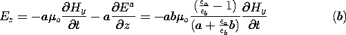
| 14.8.4* | The transmission line model for the strip line of Fig. 14.8.4a is
derived in Prob. 14.1.1. Because the permittivity is not uniform
over the cross-section of the line, the waves represented by the
model are not exactly TEM. The approximation is valid as long as the
wavelength is long enough so that (25) is satisfied. In the
approximation, Ex is taken as being uniform with x in each of
the dielectrics, Ea and Eb, respectively. To estimate the
longitudinal field Ez and compare it to Ea,
an incremental surface between z + z and z and between the
perfect conductors to derive Faraday's transmission line equation
written in terms of Ea.

| ||||||||
Quasi-One-Dimensional Models (G = 0) | |||||||||
| 14.9.1 | The transmission line of Fig. 14.2.2a is comprised of wires having a
finite conductivity , with the dielectric between of
negligible conductivity. With the distribution of V and I
described by (7) and (10), what are C, L, and R, and over what
frequency range is this model valid? (Note Examples 4.6.3 and
8.6.1.) Give a condition on the dimensions R  a and l that
must be satisfied to have the model be self-consistent over
frequencies ranging from where the resistance dominates to where the
inductive reactance dominates. a and l that
must be satisfied to have the model be self-consistent over
frequencies ranging from where the resistance dominates to where the
inductive reactance dominates.
| ||||||||
| 14.9.2 | In the coaxial transmission line of Fig. 14.2.2b, the outer conductor
has a thickness . Each conductor has the conductivity .
What are C, L, and R, and over what frequency range are (7) and
(10) valid? Give a condition on the transverse dimensions that
insures the model being valid into the frequency range where the
inductive reactance dominates the resistance.
| ||||||||
| 14.9.3 | Find V(z, t) on the charge diffusion line of Fig. 14.9.4 in the case where the applied voltage has been zero for t < 0 and suddenly becomes Vp = constant for 0 < t and the line is shorted at z = 0. (Note Example 10.6.1.) | ||||||||
| 14.9.4 | Find V(z, t) under the conditions of Prob. 14.9.3 but with the line
"open circuited" at z = 0.
|

 = lL/Rg, the current
I(0, t) found in (a) approaches that predicted by the MQS model.
= lL/Rg, the current
I(0, t) found in (a) approaches that predicted by the MQS model.