4.1
Irrotational Field Represented by Scalar Potential: TheGradient Operator and Gradient Integral Theorem

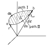
The integral of an irrotational electric field from some reference point r_ref to the position r is independent of the integration path. This follows from an integration of (1) over the surface S spanning the contour defined by alternative paths I and II, shown in Fig. 4.1.1. Stokes' theorem, (2.5.4), gives

Figure 4.1.1 Paths I and II between positions r and r_ref are spanned by surface S.

Stokes' theorem employs a contour running around the surface in a single direction, whereas the line integrals of the electric field from r to r_ref, from point a to point b, run along the contour in opposite directions. Taking the directions of the path increments into account, (1) is equivalent to

and thus, for an irrotational field, the EMF between two points is independent of path.

A field that assigns a unique value of the line integral between two points independent of path of integration is said to be conservative.

With the understanding that the reference point is kept fixed, the integral is a scalar function of the integration endpoint r. We use the symbol (r ) to define this scalar function

and call (r) the electric potential of the point r with respect to the reference point. With the endpoints consisting of "nodes" where wires could be attached, the potential difference of (1) would be the voltage at r relative to that at the reference. Typically, the latter would be the "ground" potential. Thus, for an irrotational field, the EMF defined in Sec. 1.6 becomes the voltage at the point a relative to point b.

We shall show that specification of the scalar function (r) contains the same information as specification of the field E (r). This is a remarkable fact because a vector function of r requires, in general, the specification of three scalar functions of r, say the three Cartesian components of the vector function. On the other hand, specification of (r) requires one scalar function of r.

Note that the expression (r) = constant represents a surface in three dimensions. A familiar example of such an expression describes a spherical surface having radius R.

Surfaces of constant potential are called equipotentials.

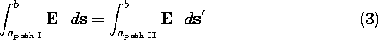
Shown in Fig. 4.1.2 are the cross-sections of two equipotential surfaces, one passing through the point r, the other through the point r + r. With r taken as a differential vector, the potential at the point r + r differs by the differential amount from that at r. The two equipotential surfaces cannot intersect. Indeed, if they intersected, both points r and r + r would have the same potential, which is contrary to our assumption.

Figure 4.1.2Two equipotential surfaces shown cut by a plane containing their normal, n.

Illustrated in Fig. 4.1.2 is the shortest distance n from the point r to the equipotential at r + r. Because of the differential geometry assumed, the length element n is perpendicular to both equipotential surfaces. From Fig. 4.1.2, n = cos r, and we have

The vector r in (6) is of arbitrary direction. It is also of arbitrary differential length. Indeed, if we double the distance n, we double and r; / n remains unchanged and thus (6) holds for any r (of differential length). We conclude that (6) assigns to every differential vector length element r, originating from r, a scalar of magnitude proportional to the magnitude of r and to the cosine of the angle between r and the unit vector n. This assignment of a scalar to a vector is representable as the scalar product of the vector length element r with a vector of magnitude / n and direction n. That is, (6) is equivalent to

where the gradient of the potential is defined as

Because it is independent of any particular coordinate system, (8) provides the best way to conceptualize the gradient operator. The same equation provides the algorithm for expressing grad in any particular coordinate system. Consider, as an example, Cartesian coordinates. Thus,

and an alternative to (6) for expressing the differential change in is

In view of (9), this expression is

and it follows that in Cartesian coordinates the gradient operation, as defined by (7), is

Here, the del operator defined by (2.1.6) is introduced as an alternative way of writing the gradient operator.

Problems at the end of this chapter serve to illustrate how the gradient is similarly determined in other coordinates, with results summarized in Table I at the end of the text.

We are now ready to show that the potential function (r ) defines E (r ) uniquely. According to (4), the potential changes from the point r to the point r + r by

The first two integrals in (13) follow from the definition of , (4). By recognizing that ds is r and that r is of differential length, so that E (r) can be considered constant over the length of the vector r, it can be seen that the last integral in (13) becomes

The vector element r is arbitrary. Therefore, comparison of (14) to (7) shows that

Given the potential function (r), the associated electric field intensity is the negative gradient of .

Note that we also obtained a useful integral theorem, for if (15) is substituted into (4), it follows that

That is, the line integration of the gradient of is simply the difference in potential between the endpoints. Of course, can be any scalar function.

In retrospect, we can observe that the representation of E by (15) guarantees that it is irrotational, for the vector identity holds

The curl of the gradient of a scalar potential vanishes. Therefore, given an electric field represented by a potential in accordance with (15), (4.0.1) is automatically satisfied.

Because the preceding discussion shows that the potential contains full information about the field E, the replacement of E by grad ( ) constitutes a general solution, or integral, of (4.0.1). Integration of a first-order ordinary differential equation leads to one arbitrary integration constant. Integration of the first-order vector differential equation curl E = 0 yields a scalar function of integration, (r ).

Thus far, we have not made any specific assignment for the reference point r_ref. Provided that the potential behaves properly at infinity, it is often convenient to let the reference point be at infinity. There are some exceptional cases for which such a choice is not possible. All such cases involve problems with infinite amounts of charge. One such example is the field set up by a charge distribution that extends to infinity in the z directions, as in the second Illustration in Sec. 1.3. The field decays like 1/r with radial distance r from the charged region. Thus, the line integral of E, (4), from a finite distance out to infinity involves the difference of ln r evaluated at the two endpoints and becomes infinite if one endpoint moves to infinity. In problems that extend to infinity but are not of this singular nature, we shall assume that the reference is at infinity.

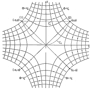
Example 4.1.1. Equipotential Surfaces

Consider the potential function (x, y), which is independent of z:

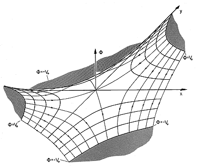
Surfaces of constant potential can be represented by a cross-sectional view in any x-y plane in which they appear as lines, as shown in Fig. 4.1.3. For the potential given by (18), the equipotentials appear in the x-y plane as hyperbolae. The contours passing through the points (a, a) and (-a, -a) have the potential V_o, while those at (a, -a) and (-a, a) have potential -V_o.

Figure 4.1.3 Cross-sectional view of surfaces of constant potential for two-dimensional potential given by (18).

The magnitude of E is proportional to the spatial rate of change of in a direction perpendicular to the constant potential surface. Thus, if the surfaces of constant potential are sketched at equal increments in potential, as is done in Fig. 4.1.3, where the increments are V_o/4, the magnitude of E is inversely proportional to the spacing between surfaces. The closer the spacing of potential lines, the higher the field intensity. Field lines, sketched in Fig. 4.1.3, have arrows that point from high to low potentials. Note that because they are always perpendicular to the equipotentials, they naturally are most closely spaced where the field intensity is largest.

Example 4.1.2. Evaluation of Gradient and Line Integral

Our objective is to exemplify by direct evaluation the fact that the line integration of an irrotational field between two given points is independent of the integration path. In particular, consider the potential given by (18), which, in view of (12), implies the electric field intensity

We integrate this vector function along two paths, shown in Fig. 4.1.3, which join points (1) and (2). For the first path, C₁, y is held fixed at y = a and hence ds = dx i_x. Thus, the integral becomes

For path C₂, y - x²/a = 0 and in general, ds = dx i_x + dy i_y, so the required integral is

However, for the path C₂ we have dy - (2x)dx/a = 0, and hence (21) becomes

Because E is found by taking the negative gradient of , and is therefore irrotational, it is no surprise that (20) and (22) give the same result.

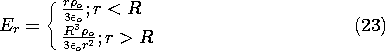
Example 4.1.3. Potential of Spherical Cloud of Charge

A uniform static charge distribution _o occupies a spherical region of radius R. The remaining space is charge free (except, of course, for the balancing charge at infinity). The following illustrates the determination of a piece-wise continuous potential function.

The spherical symmetry of the charge distribution imposes a spherical symmetry on the electric field that makes possible its determination from Gauss' integral law. Following the approach used in Example 1.3.1, the field is found to be

The potential is obtained by evaluating the line integral of (4) with the reference point taken at infinity, r = . The contour follows part of a straight line through the origin. In the exterior region, integration gives

To find in the interior region, the integration is carried through the outer region, (which gives (24) evaluated at r = R) and then into the radius r in the interior region.

Outside the charge distribution, where r R, the potential acquires the form of the coulomb potential of a point charge.

Note that q is the net charge of the distribution.

Visualization of Two-Dimensional Irrotational Fields

In general, equipotentials are three-dimensional surfaces. Thus, any two-dimensional plot of the contours of constant potential is the intersection of these surfaces with some given plane. If the potential is two-dimensional in its dependence, then the equipotential surfaces have a cylindrical shape. For example, the two-dimensional potential of (18) has equipotential surfaces that are cylinders having the hyperbolic cross-sections shown in Fig. 4.1.3.

We review these geometric concepts because we now introduce a different point of view that is useful in picturing two-dimensional fields. A three-dimensional picture is now made in which the third dimension represents the amplitude of the potential . Such a picture is shown in Fig. 4.1.4, where the potential of (18) is used as an example. The floor of the three-dimensional plot is the x - y plane, while the vertical dimension is the potential. Thus, contours of constant potential are represented by lines of constant altitude.

Figure 4.1.4 Two-dimensional potential of (18) and Fig. 4.1.3 represented in three dimensions. The vertical coordinate, the potential, is analogous to the vertical deflection of a taut membrane. The equipotentials are then contours of constant altitude on the membrane surface.

The surface of Fig. 4.1.4 can be regarded as a membrane stretched between supports on the periphery of the region of interest that are elevated or depressed in proportion to the boundary potential. By the definition of the gradient, (8), the lines of electric field intensity follow contours of steepest descent on this surface.

Potential surfaces have their greatest value in the mind's eye, which pictures a two-dimensional potential as a contour map and the lines of electric field intensity as the flow lines of water streaming down the hill.