4.2
Poisson's Equation

Given that E is irrotational, (4.0.1), and given the charge density in Gauss' law, (4.0.2), what is the distribution of electric field intensity? It was shown in Sec. 4.1 that we can satisfy the first of these equations identically by representing the vector E by the scalar electric potential .

That is, with the introduction of this relation, (4.0.1) has been integrated.

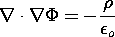
Having integrated (4.0.1), we now discard it and concentrate on the second equation of electroquasistatics, Gauss' law. Introduction of (1) into Gauss' law, (1.0.2), gives

which is identically

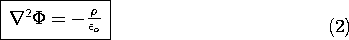
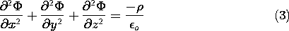
Integration of this scalar Poisson's equation, given the charge density on the right, is the objective in the remainder of this chapter.

By analogy to the ordinary differential equations of circuit theory, the charge density on the right is a "driving function." What is on the left is the operator ², denoted by the second form of (2) and called the Laplacian of . In Cartesian coordinates, it follows from the expressions for the divergence and gradient operators, (2.1.5) and (4.1.12), that

The Laplacian operator in cylindrical and spherical coordinates is determined in the problems and summarized in Table I at the end of the text. In Cartesian coordinates, the derivatives in this operator have constant coefficients. In these other two coordinate systems, some of the coefficients are space varying.

Note that in (3), time does not appear explicitly as an independent variable. Hence, the mathematical problem of finding a quasistatic electric field at the time t_o for a time-varying charge distribution (r , t) is the same as finding the static field for the time-independent charge distribution (r ) equal to (r , t = t_o), the charge distribution of the time-varying problem at the particular instant t_o.

In problems where the charge distribution is given, the evaluation of a quasistatic field is therefore equivalent to the evaluation of a succession of static fields, each with a different charge distribution, at the time of interest. We emphasize this here to make it understood that the solution of a static electric field has wider applicability than one would at first suppose: Every static field solution can represent a "snapshot" at a particular instant of time. Having said that much, we shall not indicate the time dependence of the charge density and field explicitly, but shall do so only when this is required for clarity.