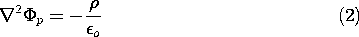
An approach to solving Poisson's equation in a region bounded by surfaces of known potential was outlined in Sec. 5.1. The potential was divided into a particular part, the Laplacian of which balances -
/
o throughout the region of interest, and a homogeneous part that makes the sum of the two potentials satisfy the boundary conditions. In short,
and on the enclosing surfaces,
The following examples illustrate this approach. At the same time they demonstrate the use of the Cartesian coordinate solutions to Laplace's equation and the idea that the fields described can be time varying.
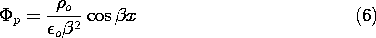
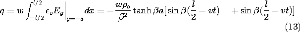
Example 5.6.1. Field of Traveling Wave of Space Charge between Equipotential Surfaces
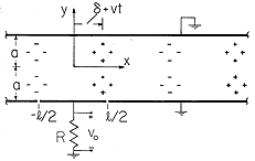
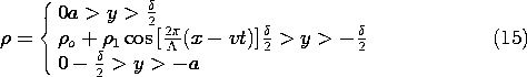
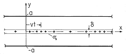
The cross-section of a two-dimensional system that stretches to infinity in the x and z directions is shown in Fig. 5.6.1. Conductors in the planes y = a and y = -a bound the region of interest. Between these planes the charge density is periodic in the x direction and uniformly distributed in the y direction.
Figure 5.6.1 Cross-section of layer of charge that is periodic in the x direction and bounded from above and below by zero potential plates. With this charge translating to the right, an insulated electrode inserted in the lower equipotential is used to detect the motion.
The parameters
are given constants. For now, the segment connected to ground through the resistor in the lower electrode can be regarded as being at the same zero potential as the remainder of the electrode in the plane x = -a and the electrode in the plane y = a. First we ask for the field distribution.
Remember that any particular solution to (2) will do. Because the charge density is independent of y, it is natural to look for a particular solution with the same property. Then, on the left in (2) is a second derivative with respect to x, and the equation can be integrated twice to obtain
This particular solution is independent of y. Note that it is not the potential that would be obtained by evaluating the superposition integral over the charge between the grounded planes. Viewed over all space, that charge distribution is not independent of y. In fact, the potential of (6) is associated with a charge distribution as given by (5) that extends to infinity in the +y and -y directions.
The homogeneous solution must make up for the fact that (6) does not satisfy the boundary conditions. That is, at the boundaries,
= 0 in (1), so the homogeneous and particular solutions must balance there.
Thus, we are looking for a solution to Laplace's equation, (3), that satisfies these boundary conditions. Because the potential has the same value on the boundaries, and the origin of the y axis has been chosen to be midway between, it is clear that the potential must be an even function of y. Further, it must have a periodicity in the x direction that matches that of (7). Thus, from the list of solutions to Laplace's equation in Cartesian coordinates in the middle column of Table 5.4.1, k =
The coefficient A is now adjusted so that the boundary conditions are satisfied by substituting (8) into (7).
Superposition of the particular solution, (7), and the homogeneous solution given by substituting the coefficient of (9) into (8), results in the desired potential distribution.
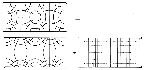
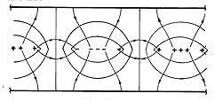
The mathematical solutions used in deriving (10) are illustrated in Fig. 5.6.2. The particular solution describes an electric field that originates in regions of positive charge density and terminates in regions of negative charge density. It is purely x directed and is therefore tangential to the equipotential boundary. The homogeneous solution that is added to this field is entirely due to surface charges. These give rise to a field that bucks out the tangential field at the walls, rendering them surfaces of constant potential. Thus, the sum of the solutions (also shown in the figure), satisfies Gauss' law and the boundary conditions.
Figure 5.6.2 Equipotentials and field lines for configuration of Fig. 5.6.1 showing graphically the superposition of particular and homogeneous parts that gives the required potential. With this static view of the fields firmly in mind, suppose that the charge distribution is moving in the x direction with the velocity v.
The variable x in (5) has been replaced by x - vt. With this moving charge distribution, the field also moves. Thus, (10) becomes
Note that the homogeneous solution is now a linear combination of the first and third solutions in the middle column of Table 5.4.1.
As the space charge wave moves by, the charges induced on the perfectly conducting walls follow along in synchronism. The current that accompanies the redistribution of surface charges is detected if a section of the wall is insulated from the rest and connected to ground through a resistor, as shown in Fig. 5.6.1. Under the assumption that the resistance is small enough so that the segment remains at essentially zero potential, what is the output voltage vo?
The current through the resistor is found by invoking charge conservation for the segment to find the current that is the time rate of change of the net charge on the segment. The latter follows from Gauss' integral law and (12) as
It follows that the dynamics of the traveling wave of space charge is reflected in a measured voltage of
In writing this expression, the double-angle formulas have been invoked.
Several predictions should be consistent with intuition. The output voltage varies sinusoidally with time at a frequency that is proportional to the velocity and inversely proportional to the wavelength, 2
/
If the charge density is concentrated in surface-like regions that are thin compared to other dimensions of interest, it is possible to solve Poisson's equation with boundary conditions using a procedure that has the appearance of solving Laplace's equation rather than Poisson's equation. The potential is typically broken into piece-wise continuous functions, and the effect of the charge density is brought in by Gauss' continuity condition, which is used to splice the functions at the surface occupied by the charge density. The following example illustrates this procedure. What is accomplished is a solution to Poisson's equation in the entire region, including the charge-carrying surface.
Example 5.6.2. Thin Bunched Charged-Particle Beam between Conducting Plates
In microwave amplifiers and oscillators of the electron beam type, a basic problem is the evaluation of the electric field produced by a bunched electron beam. The cross-section of the beam is usually small compared with a free space wavelength of an electromagnetic wave, in which case the electroquasistatic approximation applies.
We consider a strip electron beam having a charge density that is uniform over its cross-section
. The beam moves with the velocity v in the x direction between two planar perfect conductors situated at y =
a and held at zero potential. The configuration is shown in cross-section in Fig. 5.6.3. In addition to the uniform charge density, there is a "ripple" of charge density, so that the net charge density is
where
Figure 5.6.3 Cross-section of sheet beam of charge between plane parallel equipotential plates. Beam is modeled by surface charge density having dc and ac parts. The thickness
where
o =
In regions (a) and (b), respectively, above and below the beam, the potential obeys Laplace's equation. Superscripts (a) and (b) are now used to designate variables evaluated in these regions. To guarantee that the fundamental laws are satisfied within the sheet, these potentials must satisfy the jump conditions implied by the laws of Faraday and Gauss, (5.3.4) and (5.3.5). That is, at y = 0
To complete the specification of the field in the region between the plates, boundary conditions are, at y = a,
and at y = -a,
In the respective regions, the potential is split into dc and ac parts, respectively, produced by the uniform and ripple parts of the charge density.
By definition,
The dc surface charge density is independent of x, so it is natural to look for potentials that are also independent of x. From the first column in Table 5.4.1, such solutions are
The four coefficients in these expressions are determined from (17)-(20), if need be, by substitution of these expressions and formal solution for the coefficients. More attractive is the solution by inspection that recognizes that the system is symmetric with respect to y, that the uniform surface charge gives rise to uniform electric fields that are directed upward and downward in the two regions, and that the associated linear potential must be zero at the two boundaries.
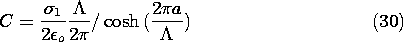
Now consider the ac part of the potential. The x dependence is suggested by (18), which makes it clear that for product solutions, the x dependence of the potential must be the cosine function moving with time. Neither the sinh nor the cosh functions vanish at the boundaries, so we will have to take a linear combination of these to satisfy the boundary conditions at y = +a. This is effectively done by inspection if it is recognized that the origin of the y axis used in writing the solutions is arbitrary. The solutions to Laplace's equation that satisfy the boundary conditions, (19) and (20), are
These potentials must match at y = 0, as required by (17), so we might just as well have written them with the coefficients adjusted accordingly.
The one remaining coefficient is determined by substituting these expressions into (18) (with
We have found the potential as a piece-wise continuous function. In region (a), it is the superposition of (24) and (28), while in region (b), it is (25) and (29). In both expressions, C is provided by (30).
When t = 0, the ac part of this potential distribution is as shown by Fig. 5.6.4. With increasing time, the field distribution translates to the right with the velocity v. Note that some lines of electric field intensity that originate on the beam terminate elsewhere on the beam, while others terminate on the equipotential walls. If the walls are even a wavelength away from the beam (a = \Lambda ), almost all the field lines terminate elsewhere on the beam. That is, coupling to the wall is significant only if the wavelength is on the order of or larger than a. The nature of solutions to Laplace's equation is in evidence. Two-dimensional potentials that vary rapidly in one direction must decay equally rapidly in a perpendicular direction.
Figure 5.6.4 Equipotentials and field lines caused by ac part of sheet charge in the configuration of Fig. 5.6.3. A comparison of the fields from the sheet beam shown in Fig. 5.6.4 and the periodic distribution of volume charge density shown in Fig. 5.6.2 is a reminder of the similarity of the two physical situations. Even though Laplace's equation applies in the subregions of the configuration considered in this section, it is really Poisson's equation that is solved "in the large," as in the previous example.