5.8
Examples in Polar Coordinates

With the objective of attaching physical insight to the polar coordinate solutions to Laplace's equation, two types of examples are of interest. First are certain classic problems that have simple solutions. Second are examples that require the generally applicable modal approach that makes it possible to satisfy arbitrary boundary conditions.

The equipotential cylinder in a uniform applied electric field considered in the first example is in the first category. While an important addition to our resource of case studies, the example is also of practical value because it allows estimates to be made in complex engineering systems, perhaps of the degree to which an applied field will tend to concentrate on a cylindrical object.

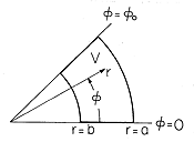
Figure 5.8.1 Natural boundaries in polar coordinates enclose region V.

In the most general problem in the second category, arbitrary potentials are imposed on the polar coordinate boundaries enclosing a region V, as shown in Fig. 5.8.1. The potential is the superposition of four solutions, each meeting the potential constraint on one of the boundaries while being zero on the other three. In Cartesian coordinates, the approach used to find one of these four solutions, the modal approach of Sec. 5.5, applies directly to the other three. That is, in writing the solutions, the roles of x and y can be interchanged. On the other hand, in polar coordinates the set of solutions needed to represent a potential imposed on the boundaries at r = a or r = b is different from that appropriate for potential constraints on the boundaries at = 0 or = _o. Examples 5.8.2 and 5.8.3 illustrate the two types of solutions needed to determine the fields in the most general case. In the second of these, the potential is expanded in a set of orthogonal functions that are not sines or cosines. This gives the opportunity to form an appreciation for an orthogonality property of the product solutions to Laplace's equation that prevails in many other coordinate systems.

Simple Solutions

The example considered now is the first in a series of "cylinder" case studies built on the same m = 1 solutions. In the next chapter, the cylinder will become a polarizable dielectric. In Chap. 7, it will have finite conductivity and provide the basis for establishing just how "perfect" a conductor must be to justify the equipotential model used here. In Chaps. 8-10, the field will be magnetic and the cylinder first perfectly conducting, then magnetizable, and finally a shell of finite conductivity. Because of the simplicity of the dipole solutions used in this series of examples, in each case it is possible to focus on the physics without becoming distracted by mathematical details.

Example 5.8.1. Equipotential Cylinder in a Uniform Electric Field

A uniform electric field E_a is applied in a direction perpendicular to the axis of a (perfectly) conducting cylinder. Thus, the surface of the conductor, which is at r = R, is an equipotential. The objective is to determine the field distribution as modified by the presence of the cylinder.

Because the boundary condition is stated on a circular cylindrical surface, it is natural to use polar coordinates. The field excitation comes from "infinity," where the field is known to be uniform, of magnitude E_a, and x directed. Because our solution must approach this uniform field far from the cylinder, it is important to recognize at the outset that its potential, which in Cartesian coordinates is -E_a x, is

To this must be added the potential produced by the charges induced on the surface of the conductor so that the surface is maintained an equipotential. Because the solutions have to hold over the entire range 0 < < 2, only integer values of the separation constant m are allowed, i.e., only solutions that are periodic in . If we are to add a function to (1) that makes the potential zero at r = R, it must cancel the value given by (1) at each point on the surface of the cylinder. There are two solutions in Table 5.7.1 that have the same cos dependence as (1). We pick the 1/r dependence because it decays to zero as r and hence does not disturb the potential at infinity already given by (1). With A an arbitrary coefficient, the solution is therefore

Because = 0 at r = R, evaluation of this expression shows that the boundary condition is satisfied at every angle if

and the potential is therefore

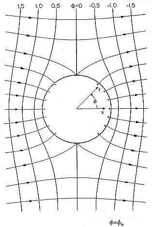
The equipotentials given by this expression are shown in Fig. 5.8.2. Note that the x = 0 plane has been taken as having zero potential by omitting an additive constant in (1). The field lines shown in this figure follow from taking the gradient of (4).

Figure 5.8.2 Equipotentials and field lines for perfectly conducting cylinder in initially uniform electric field.

Field lines tend to concentrate on the surface where = 0 and = . At these locations, the field is maximum and twice the applied field. Now that the boundary value problem has been solved, the surface charge on the cylindrical conductor follows from Gauss' jump condition, (5.3.2), and the fact that there is no field inside the cylinder.

In retrospect, the boundary condition on the circular cylindrical surface has been satisfied by adding to the uniform potential that of an x directed line dipole. Its moment is that necessary to create a field that cancels the tangential field on the surface caused by the imposed field.

Azimuthal Modes

The preceding example considered a situation in which Laplace's equation is obeyed in the entire range 0 < < 2. The next two examples illustrate how the polar coordinate solutions are adapted to meeting conditions on polar coordinate boundaries that have arbitrary locations as pictured in Fig. 5.8.1.

Example 5.8.2. Modal Analysis in : Fields in and around Corners

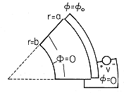
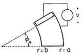
The configuration shown in Fig. 5.8.3, where the potential is zero on the walls of the region V at r = b and at = 0 and = _o, but is v on a curved electrode at r = a, is the polar coordinate analogue of that considered in Sec. 5.5. What solutions from Table 5.7.1 are pertinent? The region within which Laplace's equation is to be obeyed does not occupy a full circle, and hence there is no requirement that the potential be a single-valued function of . The separation constant m can assume noninteger values.

Figure 5.8.3 Region of interest with zero potential boundaries at = 0, = _o, and r = b and electrode at r = a having potential v.

We shall attempt to satisfy the boundary conditions on the three zero-potential boundaries using individual solutions from Table 5.7.1. Because the potential is zero at = 0, the cosine and ln(r) terms are eliminated. The requirement that the potential also be zero at = _o eliminates the functions and ln(r). Moreover, the fact that the remaining sine functions must be zero at = _o tells us that m_o = n. Solutions in the last column are not appropriate because they do not pass through zero more than once as a function of . Thus, we are led to the two solutions in the second column that are proportional to sin (n /_o).

In writing these solutions, the r's have been normalized to b, because it is then clear by inspection how the coefficients A_n and B_n are related to make the potential zero at r = b, A_n = -B_n.

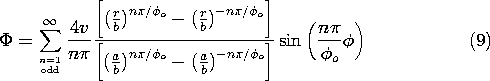
Each term in this infinite series satisfies the conditions on the three boundaries that are constrained to zero potential. All of the terms are now used to meet the condition at the "last" boundary, where r = a. There we must represent a potential which jumps abruptly from zero to v at = 0, stays at the same v up to = _o, and then jumps abruptly from v back to zero. The determination of the coefficients in (8) that make the series of sine functions meet this boundary condition is the same as for (5.5.4) in the Cartesian analogue considered in Sec. 5.5. The parameter n (x/a) of Sec. 5.5 is now to be identified with n ( /_o). With the potential given by (8) evaluated at r = a, the coefficients must be as in (5.5.17) and (5.5.18). Thus, to meet the "last" boundary condition, (8) becomes the desired potential distribution.

The distribution of potential and field intensity implied by this result is much like that for the region of rectangular cross-section depicted in Fig. 5.5.3. See Fig. 5.8.3.

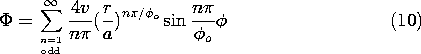
In the limit where b 0, the potential given by (9) becomes

and describes the configurations shown in Fig. 5.8.4. Although the wedge-shaped region is a reasonable "distortion" of its Cartesian analogue, the field in a region with an outside corner ( /_o < 1) is also represented by (10). As long as the leading term has the exponent /_o > 1, the leading term in the gradient [with the exponent ( /_o) - 1] approaches zero at the origin. This means that the field in a wedge with _o < approaches zero at its apex. However, if /_o < 1, which is true for < _o < 2 as illustrated in Fig. 5.8.4b, the leading term in the gradient of has the exponent ( /_o) - 1 < 0, and hence the field approaches infinity as r 0. We conclude that the field in the neighborhood of a sharp edge is infinite. This observation teaches a lesson for the design of conductor shapes so as to avoid electrical breakdown. Avoid sharp edges!

Figure 5.8.4 Pie-shaped region with zero potential boundaries at = 0 and = _o and electrode having potential v at r = a. (a) With included angle less than 180 degrees, fields are shielded from region near origin. (b) With angle greater than 180 degrees, fields tend to concentrate at origin.

Radial Modes

The modes illustrated so far possessed sinusoidal dependencies, and hence their superposition has taken the form of a Fourier series. To satisfy boundary conditions imposed on constant planes, it is again necessary to have an infinite set of solutions to Laplace's equation. These illustrate how the product solutions to Laplace's equation can be used to provide orthogonal modes that are not Fourier series.

To satisfy zero potential boundary conditions at r = b and r = a, it is necessary that the function pass through zero at least twice. This makes it clear that the solutions must be chosen from the last column in Table 5.7.1. The functions that are proportional to the sine and cosine functions can just as well be proportional to the sine function shifted in phase (a linear combination of the sine and cosine). This phase shift is adjusted to make the function zero where r = b, so that the radial dependence is expressed as

and the function made to be zero at r = a by setting

where n is an integer.

The solutions that have now been defined can be superimposed to form a series analogous to the Fourier series.

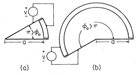
For a/b = 2, the first three terms in the series are illustrated in Fig. 5.8.5. They have similarity to sinusoids but reflect the polar geometry by having peaks and zero crossings skewed toward low values of r.

Figure 5.8.5 Radial distribution of first three modes given by (13) for a/b = 2. The n = 3 mode is the radial dependence for the potential shown in Fig. 5.7.6.

With a weighting function g(r) = r^-1, these modes are orthogonal in the sense that

It can be shown from the differential equation defining R(r), (5.7.5), and the boundary conditions, that the integration gives zero if the integration is over the product of different modes. The proof is analogous to that given in Cartesian coordinates in Sec. 5.5.

Consider now an example in which these modes are used to satisfy a specific boundary condition.

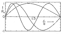
Example 5.8.3. Modal Analysis in r

The region of interest is of the same shape as in the previous example. However, as shown in Fig. 5.8.6, the zero potential boundary conditions are at r = a and r = b and at = 0. The "last" boundary is now at = _o, where an electrode connected to a voltage source imposes a uniform potential v.

Figure 5.8.6 Region with zero potential boundaries at r = a, r = b, and = 0. Electrode at = _o has potential v.

The radial boundary conditions are satisfied by using the functions described by (13) for the radial dependence. Because the potential is zero where = 0, it is then convenient to use the hyperbolic sine to represent the dependence. Thus, from the solutions in the last column of Table 5.7.1, we take a linear combination of the second and fourth.

Using an approach that is analogous to that for evaluating the Fourier coefficients in Sec. 5.5, we now use (15) on the "last" boundary, where = _o and = v, multiply both sides by the mode R_m defined with (13) and by the weighting factor 1/r, and integrate over the radial span of the region.

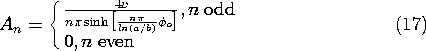
Out of the infinite series on the right, the orthogonality condition, (14), picks only the m-th term. Thus, the equation can be solved for A_m and m n. With the substitution u = m ln(r/b)/ln(a/b), the integrals can be carried out in closed form.

A picture of the potential and field intensity distributions represented by (15) and its negative gradient is visualized by "bending" the rectangular region shown by Fig. 5.5.3 into the curved region of Fig. 5.8.6. The role of y is now played by .