5.9
Three Solutions to Laplace's Equation inSpherical Coordinates

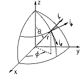
The method employed to solve Laplace's equation in Cartesian coordinates can be repeated to solve the same equation in the spherical coordinates of Fig. 5.9.1. We have so far considered solutions that depend on only two independent variables. In spherical coordinates, these are commonly r and . These two-dimensional solutions therefore satisfy boundary conditions on spheres and cones.

Figure 5.9.1 Spherical coordinate system.

Rather than embark on an exploration of product solutions in spherical coordinates, attention is directed in this section to three such solutions to Laplace's equation that are already familiar and that are remarkably useful. These will be used to explore physical processes ranging from polarization and charge relaxation dynamics to the induction of magnetization and eddy currents.

Under the assumption that there is no dependence, Laplace's equation in spherical coordinates is (Table I)

The first of the three solutions to this equation is independent of and is the potential of a point charge.

If there is any doubt, substitution shows that Laplace's equation is indeed satisfied. Of course, it is not satisfied at the origin where the point charge is located.

Another of the solutions found before is the three-dimensional dipole, (4.4.10).

This solution factors into a function of r alone and of alone, and hence would have to turn up in developing the product solutions to Laplace's equation in spherical coordinates. Substitution shows that it too is a solution of (1).

The third solution represents a uniform z-directed electric field in spherical coordinates. Such a field has a potential that is linear in z, and in spherical coordinates, z = r cos . Thus, the potential is

These last two solutions, for the three-dimensional dipole at the origin and a field due to charges at z , are similar to those for dipoles in two dimensions, the m = 1 solutions that are proportional to cos from the second column of Table 5.7.1. However, note that the two-dimensional dipole potential varies as r^-1, while the three dimensional dipole potential has an r^-2 dependence. Also note that whereas the polar coordinate dipole can have an arbitrary orientation (can be a sine as well as a cosine function of , or any linear combination of these), the three-dimensional dipole is z directed. That is, do not replace the cosine function in (3) by a sine function and expect that the potential will satisfy Laplace's equation in spherical coordinates.

Example 5.9.1. Equipotential Sphere in a Uniform Electrical Field

Consider a raindrop in an electric field. If in the absence of the drop, that field is uniform over many drop radii R, the field in the vicinity of the drop can be computed by taking the field as being uniform "far from the sphere." The field is z directed and has a magnitude E_a. Thus, on the scale of the drop, the potential must approach that of the uniform field (4) as r .

We will see in Chap. 7 that it takes only microseconds for a water drop in air to become an equipotential. The condition that the potential be zero at r = R and yet approach the potential of (5) as r is met by adding to (5) the potential of a dipole at the origin, an adjustable coefficient times (3). By writing the r dependencies normalized to the drop radius R, it is possible to see directly what this coefficient must be. That is, the proposed solution is

and it is clear that to make this function zero at r = R, A = -1.

Note that even though the configuration of a perfectly conducting rod in a uniform transverse electric field (as considered in Example 5.8.1) is very different from the perfectly conducting sphere in a uniform electric field, the potentials are deduced from very similar arguments, and indeed the potentials appear similar. In cross-section, the distribution of potential and field intensity is similar to that for the cylinder shown in Fig. 5.8.2. Of course, their appearance in three-dimensional space is very different. For the polar coordinate configuration, the equipotentials shown are the cross-sections of cylinders, while for the spherical drop they are cross-sections of surfaces of revolution. In both cases, the potential acquired (by the sphere or the rod) is that of the symmetry plane normal to the applied field.

The surface charge on the spherical surface follows from (7).

Thus, for E_a > 0, the north pole is capped by positive surface charge while the south pole has negative charge. Although we think of the second solution in (7) as being due to a fictitious dipole located at the sphere's center, it actually represents the field of these surface charges. By contrast with the rod, where the maximum field is twice the uniform field, it follows from (8) that the field intensifies by a factor of three at the poles of the sphere.

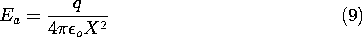
In making practical use of the solution found here, the "uniform field at infinity E_a" is that of a field that is slowly varying over dimensions on the order of the drop radius R. To demonstrate this idea in specific terms, suppose that the imposed field is due to a distant point charge. This is the situation considered in Example 4.6.4, where the field produced by a point charge and a conducting sphere is considered. If the point charge is very far away from the sphere, its field at the position of the sphere is essentially uniform over the region occupied by the sphere. (To relate the directions of the fields in Example 4.6.4 to the present case, mount the = 0 axis from the center of the sphere pointing towards the point charge. Also, to make the field in the vicinity of the sphere positive, make the point charge negative, q -q.)

At the sphere center, the magnitude of the field intensity due to the point charge is

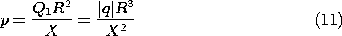
The magnitude of the image charge, given by (4.6.34), is

and it is positioned at the distance D = R²/X from the center of the sphere. If the sphere is to be charge free, a charge of strength -Q₁ has to be mounted at its center. If X is very large compared to R, the distance D becomes small enough so that this charge and the charge given by (10) form a dipole of strength

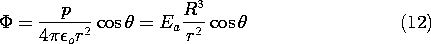
The potential resulting from this dipole moment is given by (4.4.10), with p evaluated using this moment. With the aid of (9), the dipole field induced by the point charge is recognized as

As witnessed by (7), this potential is identical to the one we have found necessary to add to the potential of the uniform field in order to match the boundary conditions on the sphere.

Of the three spherical coordinate solutions to Laplace's equation given in this section, only two were required in the previous example. The next makes use of all three.

Example 5.9.2. Charged Equipotential Sphere in a Uniform Electric Field

Suppose that the highly conducting sphere from Example 5.9.1 carries a net charge q while immersed in a uniform applied electric field E_a. Thunderstorm electrification is evidence that raindrops are often charged, and E_a could be the field they generate collectively.

In the absence of this net charge, the potential is given by (7). On the boundary at r = R, this potential remains uniform if we add the potential of a point charge at the origin of magnitude q.

The surface potential has been raised from zero to q/4_o R, but this potential is independent of and so the tangential electric field remains zero.

The point charge is, of course, fictitious. The actual charge is distributed over the surface and is found from (13) to be

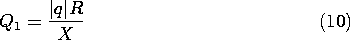
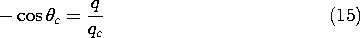
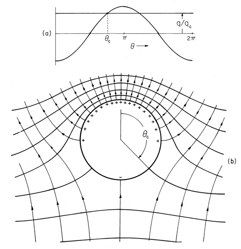
The surface charge density switches sign when the term in parentheses vanishes, when q/q_c < 1 and

Figure 5.9.2a is a graphical solution of this equation. For E_a and q positive, the positive surface charge capping the sphere extends into the southern hemisphere. The potential and electric field distributions implied by (13) are illustrated in Fig. 5.9.2b. If q exceeds q_c 12 _o E_a R², the entire surface of the sphere is covered with positive surface charge density and E is directed outward over the entire surface.

Figure 5.9.2 (a) Graphical solution of (15) for angle _c at which electric field switches from being outward to being inward directed on surface of sphere. (b) Equipotentials and field lines for perfectly conducting sphere having net charge $q$ in an initially uniform electric field.