Usually, the polarization depends on the electric field intensity. However, in some materials a permanent polarization is "frozen" into the material. Ideally, this means that P (r , t) is prescribed, independent of E. Electrets, used to make microphones and telephone speakers, are often modeled in this way.
With P a given function of space, and perhaps of time, the polarization charge density and surface charge density follow from (6.2.2) and (6.2.4) respectively. If the unpaired charge density is also given throughout the material, the total charge density in Gauss' law and surface charge density in the continuity condition for Gauss' law are known. [The right-hand sides of (6.2.1) and (6.2.3) are known.] Thus, a description of permanent polarization problems follows the same format as used in Chaps. 4 and 5.
Examples in this section are intended to develop an appreciation for the relationship between the polarization density P, the polarization charge density
p, and the electric field intensity E. It should be recognized that once
The distinction between paired and unpaired charges is sometimes academic. By subjecting an insulating material to an extremely large field, especially at an elevated temperature, it is possible to coerce molecules or domains of molecules into a polarization state that is retained for some period of time at lower fields and temperatures. It is natural to take this as a state of permanent polarization. But, if ions are made to impact the surface of the material, they can form sites of permanent charge. Certainly, the origin of these ions suggests that they be regarded as unpaired. Yet if the material attracts other charges to become neutral, as it tends to do, these permanent charges could also be regarded as due to polarization and represented by a permanent polarization charge density.
In this section, the EQS laws prevail. Thus, with the understanding that throughout the region of interest (exclusive of enclosing boundaries) the charge densities are given,
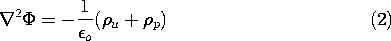
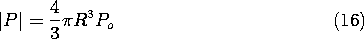
The example now considered is akin to that pictured qualitatively in Fig. 6.1.2. By making the uniformly polarized material spherical, it is possible to obtain a simple solution for the field distribution.
Example 6.3.1. A Permanently Polarized Sphere
A sphere of material having radius R is uniformly polarized along the z axis,
Given that the surrounding region is free space with no additional field sources, what is the electric field intensity E produced by this permanent polarization?
The first step is to establish the distribution of
Abrupt changes of the normal component of P entail polarization surface charge densities. These follow from using (4) to evaluate the continuity condition of (6.2.4) applied at r = R, where the normal component is ir and region (a) is outside the sphere.
This surface charge density gives rise to E.
Now that the field sources have been identified, the situation reverts to one much like that illustrated by Problem 5.9.2. Both within the sphere and in the surrounding free space, the potential must satisfy Laplace's equation, (2), with
the continuity conditions at r = R implied by (1) and (2) [(5.3.3) and (6.2.3)] with the latter evaluated using (5) are
where (o) and (i) denote the regions outside and inside the sphere.
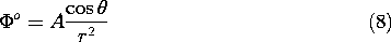
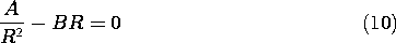
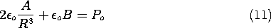
The source of the E field represented by this potential is a surface polarization charge density that varies cosinusoidally with
. It is possible to fulfill the boundary conditions, (6) and (7), with the two spherical coordinate solutions to Laplace's equation (from Sec. 5.9) having the

. Of the two possible solutions having the cos
Inside the sphere, the potential must be finite, so this solution is excluded. The solution is
which is that of a uniform electric field intensity. Substitution of these expressions into the continuity conditions, (6) and (7), gives expressions from which cos
These expressions can be solved for A and B, which are introduced into (8) and (9) to give the potential distribution
Finally, the desired distribution of electric field is obtained by taking the negative gradient of this potential.
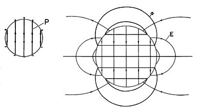
With the distribution of polarization density shown in the inset, Fig. 6.3.1 shows this electric field intensity. It comes as no surprise that the E lines originate on the positive charge and terminate on the negative. The polarization density originates on negative polarization charge and terminates on positive polarization charge. The resulting electric field is classic because outside it is exactly that of a dipole at the origin, while inside it is uniform.
Figure 6.3.1 Equipotentials and lines of electric field intensity of permanently polarized sphere having uniform polarization density. Inset shows polarization density and associated surface polarization charge density. What would be the moment of the dipole at the origin giving rise to the same external field as the uniformly polarized sphere? This can be seen from a comparison of (12) and (4.4.10).
The moment is simply the volume multiplied by the uniform polarization density.
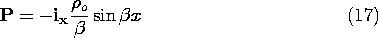
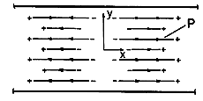
There are two new ingredients in the next example. First, the region of interest has boundaries upon which the potential is constrained. Second, the given polarization density represents a volumetric distribution of polarization charge density rather than a surface distribution.
Example 6.3.2. Fields Due to Volume Polarization Charge with Boundary Conditions
Plane parallel electrodes, in the planes y =
a, are constrained to zero potential. In the planar region between, the polarization density is the spatially periodic function
We wish to determine the field distribution.
First, the distribution of polarization charge density is determined by taking the negative divergence of (17) [(17) is substituted into (6.1.6)].
The distribution of polarization density and polarization charge density which has been found is shown in Fig. 6.3.2 (
Figure 6.3.2 Periodic distribution of polarization density and associated polarization charge density ( Now the situation reverts to solving Poisson's equation, given this source distribution and subject to the zero potential conditions on the boundaries at y =
The next example illustrates how a permanent polarization can conspire with a mechanical deformation to produce a useful electrical signal.
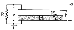
Example 6.3.3. An Electret Microphone
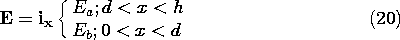
Shown in cross-section in Fig. 6.3.3 is a thin sheet of permanently polarized material having thickness d. It is bounded from below by a fixed electrode having the potential v and from above by an air gap. On the other side of this gap is a conducting grounded diaphragm which serves as the movable element of a microphone. It is mounted so that it can undergo displacements. Thus, the spacing h = h(t). Given h(t), what is the voltage developed across a load resistance R?
Figure 6.3.3 Cross-section of electret microphone. In the sheet, the polarization density is uniform, with magnitude Po, and directed from the lower electrode toward the upper one. This vector has no divergence, and so evaluation of (6.1.6) shows that the polarization charge density is zero in the volume of the sheet. The polarization surface charge density on the electret air gap interface follows from (6.1.7) as
Because
sp is uniform and the equipotential boundaries are plane and parallel, the electric field in the air gap [region (a)] and in the electret [region (b)] are taken as uniform.
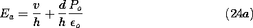
Formally, we have just solved Laplace's equation in each of the bulk regions. The fields Ea and Eb must satisfy two conditions. First, the potential difference between the electrodes is v, so
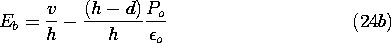
Second, Gauss' jump condition at the electret air gap interface, (6.2.3), requires that
Simultaneous solution of these last two expressions evaluates the electric fields in terms of v and h.
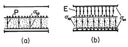
What has been found is illustrated in Fig. 6.3.4. The uniform P and associated
o > v. In the air gap, the field due to the unpaired charges on the electrodes reinforces that due to
Figure 6.3.4 (a) Distribution of polarization density and surface charge density in electret microphone. (b) Electric field intensity and surface polarization and unpaired charges. To compute the current i, defined in Fig. 6.3.3, the lower electrode and the electret are enclosed by a surface S, and Gauss' law is used to evaluate the enclosed unpaired charge.
Just how the surface S cuts through the system does not matter. Here we take the surface as enclosing the lower electrode by passing through the air gap. It follows from (24) that the unpaired charge is
where A is the area of the electrode.
Conservation of unpaired charge requires that the current be the rate of change of the total unpaired charge on the lower electrode.
With the resistor attached to the terminals (the input resistance of an amplifier driven by the microphone), the voltage and current must also satisfy Ohm's law.
These last three relations combine to give an expression for v(t), given h(t).
This differential equation has time-varying coefficients. Not only is this equation difficult to solve, but also the predicted voltage response cannot be a good replica of h(t), as required for a good microphone, if all terms are of equal importance. That situation can be remedied if the deflections h1 are kept small compared with the equilibrium position, ho
h1. In the absence of a time variation of h1, it is clear from (29) that v is zero. By making h1 small, we can make v small.
Expanding the right-hand side of (29) to first order in h1, dh1/dt, v, and dv/dt, we obtain
where Co = A
We could solve this equation for its response to a sinusoidal drive. Alternatively, the resulting frequency response can be determined, with more physical insight, by considering two limits. First, suppose that time rate of change is so slow (frequencies so low) that the first term on the left is negligible compared to the second. Then the output voltage is
In this limit, the resistor acts as a short. The charge can be determined by the diaphragm displacement with the contribution of v ignored (i.e., the charge required to produce v by charging the capacitance Co is ignored). The small but finite voltage is then obtained as the time rate of change of the charge multiplied by -R.
Second, suppose that time rates of change are so rapid that the second term is negligible compared to the first. Within an integration constant,
In this limit, the electrode charge is essentially constant. The voltage is obtained from (26) with q set equal to its equilibrium value, (A
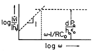
The frequency response gleaned from these asymptotic responses is in Fig. 6.3.5.
Figure 6.3.5 Frequency response of electret microphone for imposed diaphragm displacement. Because its displacement was taken as known, we have been able to ignore the dynamical equations of the diaphragm. If the mass and damping of the diaphragm are ignored, the displacement indeed reflects the pressure of a sound wave. In this limit, a linear distortion-free response of the microphone to pressure is assured at frequencies
> 1/RC. However, in predicting the response to a sound wave, it is usually necessary to include the detailed dynamics of the diaphragm.
In a practical microphone, subjecting the electret sheet to an electric field would induce some polarization over and beyond the permanent component Po. Thus, a more realistic model would incorporate features of the linear dielectrics introduced in Sec. 6.4.