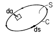
We have found that many interesting MQS cases can be treated by the use of the scalar potential obeying Laplace's equation. The vector potential, defined by (8.1.1), is necessary when analyzing fields with nonzero curl. There are other cases as well in which its use may be advantageous. The vector potential is the natural variable for evaluating the flux passing through a surface. In view of (8.1.1), integration of the flux density over the open surface S of Fig. 8.6.1 gives
Figure 8.6.1 Open surface S having area element da enclosed by contour C having directed differential length ds.
and it follows from Stokes' theorem that this flux is equal to the line integral of A
ds around the contour enclosing the surface.
In certain important cases, A has only one component and a vector field is again represented in terms of one scalar function. Two such cases are identified in the following subsections.
Vector Potential for Two-Dimensional Fields
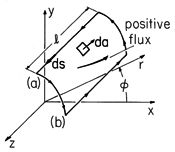
Suppose that the flux density is parallel to the x - y plane and is independent of z. It can then be represented by a vector potential having only a z component.
Note that the divergence of this A is automatically zero and that in Cartesian coordinates, the components of the flux density are given in terms of Az by
Figure 8.6.2 Surface S with sides of length l parallel to the z axis at locations (a) and (b). The contour direction is consistent with the flux being positive, as shown.
Consider now the evaluation of the net flux of magnetic flux density through a surface S that has length l in the z direction, as shown in Fig. 8.6.2. The points (a) and (b) denote the coordinates of the corners of the contour enclosing S. The contour consists of a pair of parallel straight segments of length l parallel to the z axis, one at the location (a) in the x - y plane and the other at (b), and contours joining (a) and (b) in x - y planes. Contributions to the contour integral, (2), from these latter segments of C are zero, because A is perpendicular to ds. Integration along the z-directed segments amounts to multiplication of Az evaluated at (a) or (b) by the length of the segment. Thus, (1) becomes
The vector potential at (a) relative to (b) is the net magnetic flux per unit length passing through a surface of unit length in the z direction subtended between the two points and a corresponding pair at unity distance along the z axis. Note that the flux has a sign, relative to the direction of the contour integration, governed by the right-hand rule (Fig. 1.4.1).
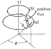
Vector Potential for Axisymmetric Fields in Spherical Coordinates
If the magnetic flux density is invariant with respect to rotation around the z axis, having components in the r and
directions only, the vector potential again has a single component.
The net flux through the annular surface "spanned" over the contour shown in Fig. 8.6.3, having constant outer and inner radii denoted by (a) and (b), respectively, is given by the contributions to (2) of the azimuthal segments, A
multiplied by the circumferences. The contour is closed by adjacent oppositely directed segments joining points (a) and (b) in a plane of constant
at (a) relative to that at (b).
5 With A used to represent the velocity distribution of an incompressible fluid,) is called Stokes' stream function.
Figure 8.6.3 Difference between axisymmetric stream function
where
Lines of flux density are tangential to the axisymmetric surfaces of constant
Boundary Value Solution by "Inspection"
In two-dimensional configurations, any surface of constant Az can be replaced by the surface of a perfect conductor. Moreover, in the free space region between conductors, Az satisfies Laplace's equation. Thus, any two-dimensional configuration from Chaps. 4 and 5 can be replaced by one where the potential lines are field lines. The equipotential (constant
) surfaces of the EQS perfect conductors become the perfectly conducting (constant Az) surfaces of an MQS system.
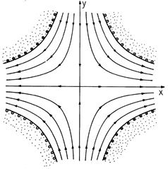
Illustration. Field Trapped between Hyperbolic Perfect Conductors
The two-dimensional potential distribution of Example 4.1.1 suggests the vector potential Az =

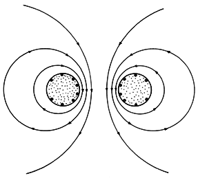
Figure 8.6.4 Surfaces of constant Az and hence lines of magnetic field intensity for field trapped between perfectly conducting electrodes. This solution is the superposition of the fields of four line currents. Two directed in the +z direction are at infinity in the first and third quadrants, while two in the -z direction are in the second and fourth quadrants.
Example 8.6.1. Field and Inductance of Oppositely Directed Currents in Parallel Perfectly Conducting Cylinders
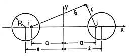
The cross-section of a pair of parallel perfectly conducting cylinders that extend to
in the z direction is shown in Fig. 8.6.5. The conductors have the same geometry as in the EQS case considered in Example 4.6.3. However, they should be regarded as shorted at one end and driven by a current source i at the other. Thus, current in the +z direction in the right conductor is returned in the left conductor. Although the net current in each conductor is given, its distribution on the surface of the conductors is to be determined.
Figure 8.6.5 Cross-section of perfectly conducting parallel conductors having radius R and spacing 2l. Fields of oppositely directed line currents having spacing 2a are shown to satisfy normal flux boundary condition on circular cylindrical surfaces of conductors. Example 4.6.3 suggests our strategy. Instead of superimposing the potentials
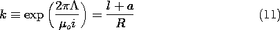
With the identification of variables
this expression is identical to that for the antidual EQS configuration, (4.6.18). We can conclude that the line currents should be located at a = (l2 - R2)1/2, and that the constant k used in that deduction (4.6.20) is identified using (10).
Here, the potential U in (4.6.20) is replaced by the flux per unit length
Figure 8.6.6 Surfaces of constant Az and hence lines of magnetic field intensity for the parallel conductor configuration shown in the same cross-sectional view by Fig. 8.6.5. The inductance per unit length L is now deduced from (11).
In the limit where the conductors represent wires that are thin compared to their spacing, the inductance per unit length of (12) is approximated using (4.6.28).
Once the vector potential has been determined, it is possible to evaluate the distribution of current density on the conductors. Note that the currents tend to concentrate on the inside surfaces of the conductors, where the magnetic field intensity is more intense.
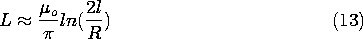
We are one step short of a general relationship between the capacitance per unit length and inductance per unit length of a pair of parallel perfect conductors, regardless of the cross-sectional geometry. With
l /
where c is the velocity of light (3.1.16).
Note that inductance per unit length of parallel circular conductors given by (12) and the capacitance per unit length for the same conductors under "open circuit" conditions (4.6.27) satisfy the general relation (14).
Method of Images
In the presence of a planar perfect conductor, the zero normal flux condition can be satisfied by symmetrically mounting source distributions on both sides of the plane. This approach is familiar from Sec. 4.7, where the boundary condition required a plane of symmetry on which the tangential electric field was zero. Here we require that the field intensity be tangential to the boundary. For two-dimensional configurations, the analogy between the electric potential and Az makes the image method of Sec. 4.7 directly applicable here. In both cases, the symmetry plane is one of constant potential (
The most obvious example is an infinitely long line current at a distance d/2 from a perfectly conducting plane. If Fig. 4.7.1 were a picture of line charges rather than point charges, this would be the dual situation. The appropriate image is then an oppositely directed line current located at a distance d/2 to the other side of the perfectly conducting plane. By making a pair of symmetrically located line currents the image for this pair of currents, the boundary condition on yet another plane can be satisfied, the analog to the configuration of Fig. 4.7.3.
The following demonstration is intended to emphasize that the perfectly conducting symmetry plane carries a surface current that terminates the field in the region of interest.
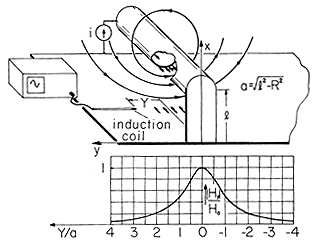
Demonstration 8.6.1. Surface Currents Induced in Ground Plane by Overhead Conductor
The metal cylinder mounted over a metal ground plane shown in Fig. 8.6.7 is familiar from Demonstration 4.7.1. Rather than being insulated from the ground plane and driven by a voltage source, this cylinder is shorted to the ground plane at one end and driven by a current source at the other. The height l is small compared to the length, so that the two-dimensional model describes the field distribution in the midregion.
Figure 8.6.7 With the frequency high enough so that the currents distribute themselves with a negligible normal flux density on the conductors, the field intensity tangential to the conducting plane is that predicted by (16) and shown by the graph. At low frequencies, the current tends to be uniformly distributed in the planar conductor. A probe is used to measure the magnetic flux density tangential to the metal ground plane. The distribution of this field, and hence of the surface current density in the adjacent metal, can be determined by recognizing that the ground plane boundary condition of no normal flux density is met by symmetrically mounting a distribution of oppositely directed currents below the metal sheet. This is just what was done in determining the fields for the pair of cylindrical conductors, Fig. 8.6.5. Thus, (9) is the image solution for the region x
0. In terms of x and y,
The flux density tangential to the ground plane at the location y = Y is
Normalized to Ho = i/
The role of the surface current density implied by this tangential field is demonstrated by the same probe measurement of the magnetic flux density normal to the conducting sheet. Provided that the frequency is high enough so that the sheet does indeed behave as a perfect conductor, this flux density is small compared to that tangential to the sheet. This is also true at the surface of the cylindrical conductor.
To appreciate the physical origins of this distribution, a dc current source is used in place of the ac source. The distribution of current in the sheet is then dictated by the rules of steady conduction, as enunciated in the first half of Chap. 7. If the sheet is long enough compared to its width, the current is uniformly distributed over the sheet and over the cross-section of the cylinder. By contrast with the high-frequency ac case, where the field is terminated by surface currents in the sheet, the magnetic field now extends below the sheet.
The method of images is not restricted to the two-dimensional situations where there is a convenient analogy between
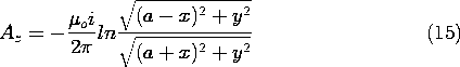
Example 8.6.2. Current Loop above a Perfectly Conducting Plane
A current loop with time-varying current i is mounted a distance h above a perfectly conducting plane, as shown in Fig. 8.6.8. Its axis is inclined at an angle
Figure 8.6.8 Current loop at distance h above a perfectly conducting plane.
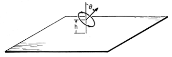
Figure 8.6.9 Cross-section of configuration of Fig. 8.6.8, showing image dipole giving rise to field that cancels the flux density normal to the planar perfect conductor. To satisfy the boundary condition in the plane of the perfectly conducting sheet, an image loop is mounted as shown in Fig. 8.6.9. For each current segment in the actual loop, there is a segment in the image loop giving rise to an oppositely directed vertical component of H. Thus, the net normal flux density in the plane of the perfect conductor is zero.
Two-Dimensional Boundary Value Problems
The vector potential of a two-dimensional field parallel to the x - y plane is z directed and thus only one scalar function describes fully the associated field, as already pointed out earlier. In problems in which currents are confined to the boundaries, the scalar potential can be used as effectively as the vector potential. The lines of steepest descent of the scalar potential are the lines of constant height of the vector potential. When the region of interest contains current distributions, then use of the vector potential is required. We shall consider both situations in the examples to follow.
Example 8.6.3. Inductive Attenuator
The cross-section of two conducting electrodes that extend to infinity in the
-shaped electrode. This current is so rapidly varying that the electrodes behave as though they were perfectly conducting. The gaps of width
insulating the electrodes from each other are small compared to the other dimensions of interest. The magnetic flux (per unit length in the z direction) passing through these gaps in the directions shown is defined as
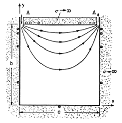
Figure 8.6.10 Cross-section of inductive attenuator. The magnetic fields are two dimensional and there are no sources in the region of interest. Thus,
oH can be represented in terms of Az, which satisfies
The walls are perfectly conducting in the sense that they are modeled as having no normal
The boundary value problem is now formally identical to the EQS capacitive attenuator that was the theme of Sec. 5.5, with the identification of variables
Thus, it follows from (5.5.9) that
The lines of magnetic flux density are the lines of constant Az. They are the equipotential "lines" of Fig. 5.5.3, shown in Fig. 8.6.10 with arrows added to indicate the field direction. Remember, there is a z-directed surface current density that is proportional to the tangential field intensity. For the flux lines shown, Kz is out of the page in the upper electrode and returned into the page on the side walls and (to an extent determined by b relative to a) on the bottom wall as well.
From the cross-sectional view given by Fig. 8.6.10, the provision for the current through the driven plate at the top to recirculate through the side and bottom plates is not shown. The following demonstration emphasizes the implied current paths at the ends of the configuration.
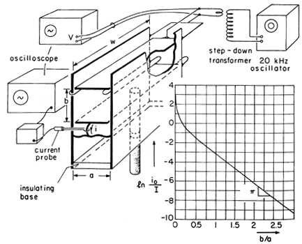
One configuration described by Example 8.6.3 is shown in Fig. 8.6.11. Here the upper plate is shorted to the adjacent walls at the near end and driven at the far end through a step-down transformer by a 20 kHz oscillator. The driving voltage v(t) at the far end of the upper plate is measured by means of an oscilloscope. The lower plate is shorted to the side walls at the far end and also connected to these walls at the near end, but in such a way that the induced current i(t) can be measured by means of a current probe.
The walls and upper and lower plates are made from brass or copper. To insure that the resistances of the plate terminations are negligible, they are made from heavy copper wire with the connections soldered. (To make it possible to adjust the spacing b, braided wire is used for the shorts on the lower electrode.)
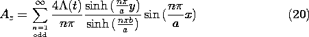
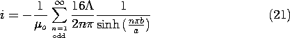
If the length w of the plates in the z direction is large compared to a and b, H within the volume follows from (20). The surface current density Kz in the lower plate then follows from evaluation of the tangential H on its surface. In turn, the total current follows from integration of Kz over the width, a, of the plate.
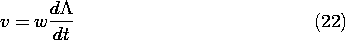
With the objective of relating this current to the driving voltage, note that (8.4.11) gives
so that with the driving voltage a sinusoid of magnitude V,
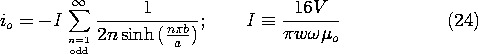
Thus, in terms of the driving voltage, the output current is io sin (
t), where it follows from (21) and (23) that
We have found that the output current, normalized to I, has the dependence on spacing between upper and lower plates shown by the inset to Fig. 8.6.11. With the spacing b small compared to a, almost all of the current through the upper plate is returned in the lower one, and the field between is essentially uniform. As the spacing b becomes comparable to the distance a between the side walls, most of the current through the upper electrode is returned in these side walls. Thus, for large b/a, the normalized output current of Fig. 8.6.11 reflects the exponential decay in the -y direction of the field.
Figure 8.6.11 Inductive attenuator demonstration. Value is added to this demonstration if it is compared to its EQS antidual, Demonstration 5.5.1. For the EQS configuration, the lower plate was properly constrained to essentially the same potential as the walls by connecting it to these side walls through a resistance (which was then used to measure the induced current). Up to frequencies above 100 Hz in the EQS case, this resistance could be as high as that of the oscilloscope (say 1 M
) and still constrain the lower plate to essentially the same zero potential as the walls. In the MQS case, we did not use a resistance to connect the lower plate to the side walls (and hence provide a means of measuring the output current), because that resistance would have had to be extremely low, even at 20 kHz, to prevent flux from leaking through the gaps between the lower plate and the side walls. We used the current probe instead. The effects of finite conductivity in MQS systems are the subject of Chap. 10.
In a final example, we exemplify how the particular and homogeneous solutions are combined to satisfy boundary conditions while also illustrating how the inductance of a distributed winding is determined.
Example 8.6.4. Field and Inductance of Distributed Winding Bounded by Perfect Conductor
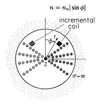
The cross-section of a distributed winding of radius a is shown in Fig. 8.6.12. It consists of turns carrying current i in the +z direction at a location (r,

Figure 8.6.12 Cross-section of two-dimensional distributed winding surrounded by perfectly conducting material. A typical coil consists of wires carrying current in the +z direction at (r, The total number of wires N in the left-hand half of the coil is
so that the current density is
The windings are very long in the z direction so that effects of the end turns are ignored and the fields taken as independent of z.
The coil is bounded at r = a by a perfect conductor. With the following steps we determine the field distribution throughout the winding and finally, its inductance.
The vector potential is z independent and must satisfy Poisson's equation (8.1.6). In polar coordinates,
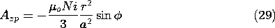
First we look for a particular solution. If it is to take a product form, inspection shows that sin
The magnetic flux density normal to the perfectly conducting surface at r = a must be zero, so the total vector potential must be constant there. It follows that one must add a vector potential with no associated current density in the region r < a, a homogeneous solution Azh. At r = a, the homogeneous solution, Azh, must be the negative of the particular solution, Azp.
A linear combination of the two solutions to Laplace's equation that have the same
The coefficient D must be zero so that the solution is finite at the origin. The coefficient C is then adjusted to make (31) satisfy the condition of (30). Hence, the sum of the particular and homogeneous solutions is
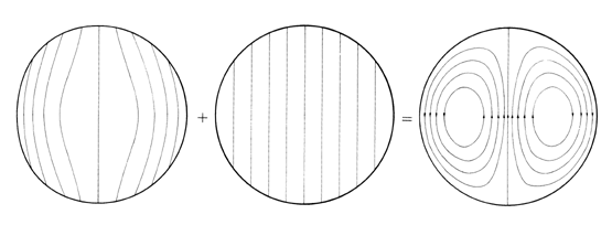
A graphical representation of what has been accomplished is given in Fig. 8.6.13, where the surfaces of constant Az (and hence the lines of field intensity) are shown for the particular, homogeneous, and total solutions.
Figure 8.6.13 Graphical representation of the surfaces of constant Az for the system of Fig. 8.6.12 as the sum of particular and homogeneous solutions. Each turn of the coil links a different magnetic flux. Thus, to determine the total flux linked by the distribution of turns, it is necessary to carry out an integration. To do this, first observe that the flux linked by the turns with their right legs within the area rd
Here, l is the length of the system in the z direction.
The total flux linked by all of the turns is obtained by integrating over all of the turns.
Substitution for Az from (32) and use of (26) then gives
where L will be recognized as the inductance.