6.02 Practice Problems: Modulation & Demodulation

Problem 1.

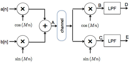
The figure below shows our "standard" modulation-demodulation system diagram: at the transmitter, signal $x[n]$ is modulated onto signal $mod[n]$ and the result $chan[n]$ is sent to the receiver, where the incoming signal is demodulated by $demod[n]$ and sent through a low-pass filter to produce $y[n]$.

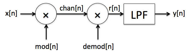
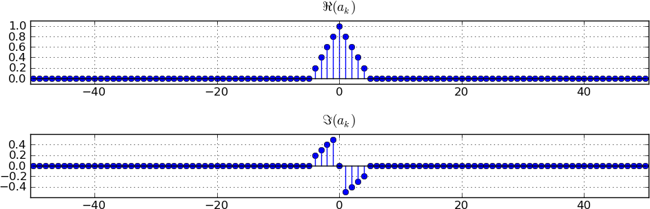
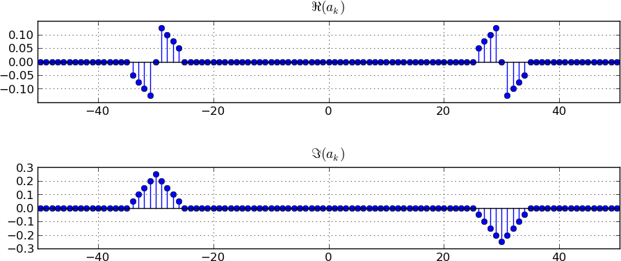
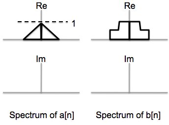
Suppose the signal $x[n]$ has a DTFT or spectrum $X(\Omega)$ whose samples $X(\Omega_k)$ at 101 points in the interval $[-\pi,\pi]$ are as shown in the plots below, though in a scaled version. Specifically, the plots show the real and imaginary parts of $a_k=X(\Omega_k)/101$, which are referred to as the spectral coefficients (note also that the points on the frequency axis are labeled by the value of $k$ rather than by $\Omega_k$, just for notational simplicity). Similarly, the spectral coefficients for any other signal are the scaled values of its DTFT at the discrete frequencies $\Omega_k$.

1. Let $mod[n] = \cos(15(2π/101)n)$. Plot the spectral coefficients for $chan[n]$, showing both the real and imaginary components. Label relevant frequencies and amplitudes.

   

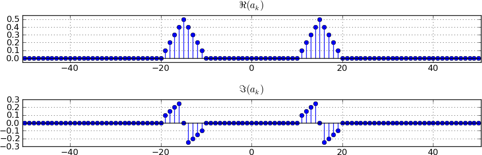
   The carrier frequency here is $\Omega_c=15(2\pi/101)=\Omega_{15}$, corresponding to $k=15$. To get the frequency domain representation of this modulated signal, we replicate the spectrum of the original signal at $-\Omega_c$ and $+\Omega_c$, scaling each of these replications by $\frac1{2}$, and adding these replications to get a single spectral plot. The basis of this result is the fact that $$\cos(\Omega_c n)=\frac1{2}\Bigl(e^{j\Omega_c n} + e^{-j\Omega_c n}\Bigr)\;.$$ The scaling of the spectrum by $\frac1{2}$ occurs because of the $\frac1{2}$ in this expression for the cosine; the replication at $+\Omega_c$ occurs because of the $e^{j\Omega_c n}$ in this expression; and the replication at $-\Omega_c$ occurs because of the $e^{-j\Omega_c n}$ in this expression. To track the details of this derivation, see Equations (14.3) and (14.4) of Chapter 14 of the class notes.

   We can carry out the process separately for the real and imaginary components of the spectrum. After carrying out these steps, we get the figures shown below. (Unfortunately the plots in the solutions to all the parts of this problem use the same symbol $a_k$ for the spectral coefficients of all the signals discussed in the problem! --- we should have actually had distinct symbols for the spectral coefficients of distinct signals.)

   

2. Let $demod[n] = \cos(15(2\pi/101)n)$, i.e., a sinusuoid of the same frequency and phase as $mod[n]$. Sketch a plot of the spectral coefficients for $r[n]$, showing both the real and imaginary components. Label relevant frequencies and amplitudes.

   

   We apply the same procedure as in part (A) above. The entire spectrum of the received signal is replicated at $-\Omega_c$ and $+\Omega_c$, scaling each by $\frac1{2}$, and adding the resulting replications. Note how the center component has twice the height of the two side components, because one copy is contributed by each of the two replications.

   

3. What ideal filtering operation on the spectrum of $y[n]$ will result in its spectral coefficients equaling those of $x[n]$?

   

   The figure above makes evident that an ideal lowpass filter with its cutoff anywhere between $\Omega_5$ and $\Omega_{25}$ (inclusive) on the positive side (and a symmetrically located cutoff on the negative side), and a gain of 2 in its pass band, will accomplish the result.

4. Let $mod[n] = \sin(15(2\pi/101)n)$, i.e., like part (A) except the modulating signal is a sine instead of a cosine. Sketch a plot of the spectral coefficients for $chan[n]$, showing both the real and imaginary components. Label relevant frequencies and amplitudes.

   

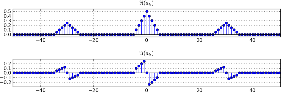
   The procedure for modulating with a sine is similar to the procedure for modulating with a cosine. However, because $$\sin(\Omega_c n)=\frac1{2j}\Bigl(e^{j\Omega_c n} - e^{-j\Omega_c n}\Bigr)=\frac{j}{2}\Bigl(e^{-j\Omega_c n} - e^{j\Omega_c n}\Bigr)\;,$$ the scaling and replication details are different: We scale the replication at $\Omega_c$ by $-j/2$ and the replication at $-\Omega_c$ by $+j/2$. This implies that the real part of the spectrum of $x[n]$ now appears in the maginary part of the spectrum of the modulated signal, and vice versa. The figure below shows the resulting spectrum. Note how the real and imaginary parts have been interchanged.

   (If you have to analyze the result of modulating a signal onto a sinusoid with arbitrary phase, you can break it up into a sine and a cosine, apply the results above for pure cosine and sine carriers, adn then combine the results appropriately.)

   

5. Let $demod[n] = \cos(15(2\pi/101)n)$, i.e., a sinusuoid of the same frequency and but $pi/2$ out of phase with $mod[n]$. Sketch a plot of the spectral coefficients for $r[n]$, showing both the real and imaginary components. Label center frequencies and peak amplitudes.

   

   This is just like part (B) except that instead of reinforcing each other, the components at the origin perfectly cancel each other out. Note how the real and imaginary parts have been interchanged.

   

6. Assuming the parameters of the LPF are set as determined in part (C), describe the spectral coefficients of $y[n]$.

   

   The spectral coefficients of $y[n]$ are now all 0. Demodulating with a signal that's $\pi/2$ out of phase with the modulating signal produces destructive addition around frequency 0.

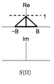
Problem 2. Single-sideband (SSB) modulation is a modulation technique designed to minimize the spectral "footprint" used to transmit an amplitude modulated signal. It takes advantage of the fact that for a real signal $s[n]$, the spectrum $S(\Omega)$ for $\Omega < 0$ can be deduced from the spectrum for $\Omega > 0$, because of the symmetry properties of $S(\Omega)$. One therefore does not need to translate all of $S(\Omega)$ to the carrier frequency, but instead only the part of the baseband spectrum corresponding to $\Omega\ge 0$. This problem leads you through one way to implement an SSB transmitter, and also treats the demodulation step.

1. Consider a band-limited signal $s[n]$ with the real triangularly shaped spectrum shown below, plotted on the $\Omega$ axis. More generally we would have had to assume that the spectrum was complex, with real part as shown, and with imaginary part given by some odd function of frequency, but we consider the case of a real spectrum here for simplicity.

   

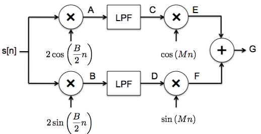
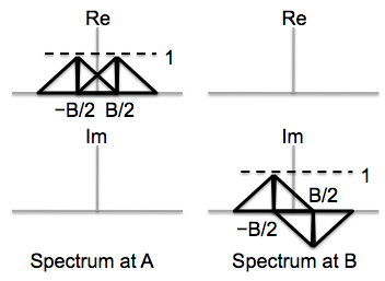
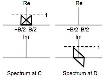
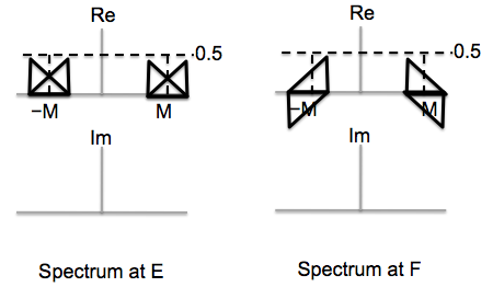
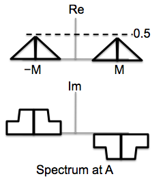
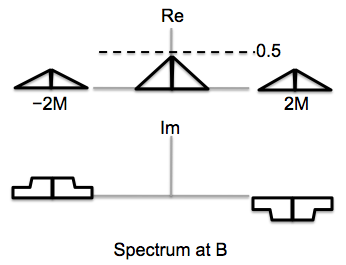
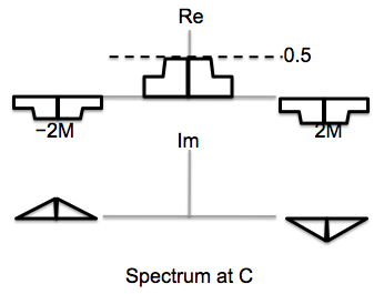
   We now modulate the signal onto two carriers, as shown in the block diagram, one phase shifted by $\pi/2$ from the other. The modulation frequency is chosen to be $B/2$, i.e., in the middle of the frequency range of the signal to be transmitted. Sketch the real and imaginary parts of the spectrum (i.e., of the DTFT) for the signals at points A and B.

   

   Use the same method as the previous question to get the spectrum of the modulated signal. Note that the two triangles overlap near the origin.

   

2. The modulated signal is now passed through a low-pass filter with a cutoff frequency of $B/2$. Sketch the real and imaginary parts of the spectrum for the signals at points C and D.

   

   Since the LPF cutoff is $B/2$, only components with frequencies between 0 and $B/2$ survive, and the rest are removed.

   

3. The signal is modulated once again to shift it up to the desired transmission frequency. Sketch the real and imaginary parts of the spectrum for the signals at points E and F.

   

   Note that both spectra have only the real part surviving. This is because C, whose spectrum is purely real, is modulated onto a cosine and thus ends up with a purely real spectrum. Similarly, D's spectrum is purely imaginary and it is modulated onto a sine, thus ending up with a spectrum that is once again real.

   

4. Finally the two signals are summed to produce the signal to be sent over the air. Sketch the real and imaginary parts of the spectrum for the signal at point G.

   

   Taking note of how subparts of the spectrum cancel when added, we end up with the following picture, in which only a a single sideband of the baseband signal is transmitted, rather than both sidebands as in normal amplitude modulation.

   

5. What operations will be needed to demodulate this signal and reconstruct the baseband signal?

   

   Demodulation proceeds as before, by modulating onto a cosine of frequency $M-\frac{B}{2}$, lowpass filtering to extract just the portion for $\Omega$ in the interval $[-B, B]$, and scaling up by a factor of 2.

Problem 3.

We learned in lecture that if we modulate a signal onto a cosine of a particular frequency, then demodulate using a sine of the same frequency and pass the result through a low-pass filter, we get nothing! We can use this effect to our advantage.

The figure below shows a so-called quadrature modulation/demodulation scheme that sends two independent signals over a single channel using the same frequency band.

The frequency axis in the spectral plots below is $\Omega$.

1. The spectra $A(\Omega)$ and $B(\Omega)$ for the signals $a[n]$ and $b[n]$ respectively are shown below. Sketch the real and imaginary parts of the spectrum for the signal at point A.

   

   

   

2. Sketch the real and imaginary parts of the spectrum for the signal at point B, right after we demodulate the combined signal using a cosine. The result is passed through a low-pass filter with a cutoff of $M$; compare the signal at point D to the two input signals and summarize your findings.

   

   The signal at point D is a scaled replica of $a[n]$.

   

3. Sketch the real and imaginary parts of the spectrum for the signal at point C, right after we demodulate the combined signal using a sine. The result is passed through a low-pass filter with a cutoff of $M$; compare the signal at point E to the two input signals and summarize your findings.

   

   The signal at point E is a scaled replica of $b[n]$.

   

Problem 4.

Consider the simple modulation-demodulation system below, which represents discrete-time (DT) signals corresponding to continuous-time (CT) signals sampled at the frequency $f_s=$10 kHz, i.e., 10,000 samples per second, and under the condition that none of the CT signals has frequency content above 5 kHz.

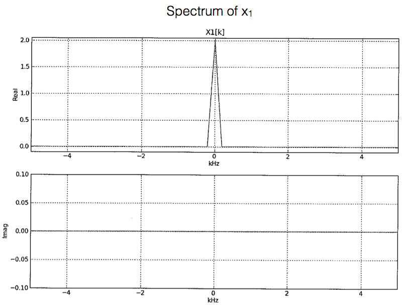
The spectrum of the input to the modulation-demodulation system is plotted below, with the frequency scale marked in Hz indicating the frequency content of the underlying continuous-time signal. Note that the spectrum is nonzero only for $|f|<100$ Hz.

Take $\Omega_a$ to correspond to a CT frequency of 1 kHz, i.e., $\Omega_a=2\pi f_a/f_s$ with $f_a=1$ kHz.

Plot the spectra of the signals at locations A and B in the above diagram. Be sure to label key features of your plot.

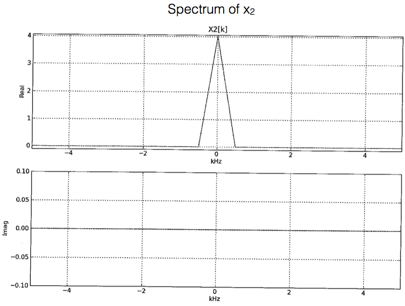
The signal is modulated onto 2 carriers, a cosine at 1 kHz and a cosine at 2 kHz. These two modulated spectra are then added up. The original signal spectrum is at the origin, so after modulation the spectral components appear at $\pm$1 kHz and $\pm$2 kHz respectively. The spectrum at A simply adds these two spectra and hence we get 4 peaks. The height of each peak is one-half that of the original and the width remains the same as in the original signal, i.e., 100 Hz.

For the spectrum at B, each of the peaks in A's spectrum is shifted and scaled by each of the carrier signals. The resulting peaks are at frequencies
2000 + 2000 = 4000
2000 - 2000 = 0
1000 + 2000 = 3000
1000 - 2000 = -1000
2000 + 1000 = 3000
2000 - 1000 = 1000
1000 + 1000 = 2000
1000 - 1000 = 0
-2000 + 2000 = 0
-2000 - 2000 = -4000
-1000 + 2000 = 1000
-1000 - 2000 = -3000
-2000 + 1000 = -1000
-2000 - 1000 = -3000
-1000 + 1000 = 0
-1000 - 1000 = -2000
Each of these is scaled down by 2 wrt the original peak height, so each of these 8 has a height of 1/4. There are two peaks at 3000, which add up to give back a height of 1/2. Similarly at -3000, -1000 and +1000. Hence, all these peaks have height 1/2. Four peaks are located at 0, and all of these add up to give a peak of height 1 at frequency 0. The remaining four are all "singleton" peaks at +/- 4000 and +/- 2000 respectively with height 1/4.

Problem 5.

All parts of this question pertain to the modulation-demodulation system shown in the figure below, where the discrete-time (DT) signals correspond to underlying continuous-time (CT) signals that are sampled at $f_s=10$ kHz (and that do not contain frequency components above 5 kHz). The carrier frequency is $f_c=500$ Hz for this problem.

1. Suppose the spectrum $Y(\Omega)$ of the signal $y[n]$ in the modulation/demodulation diagram is as plotted below.

   

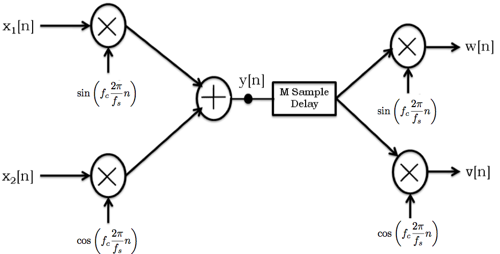
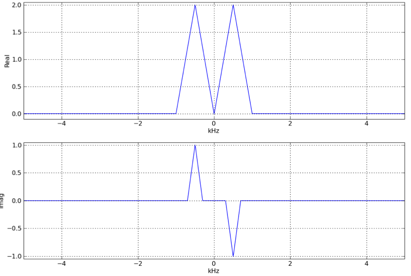
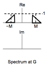
   Assuming that $M = 0$ for the $M$-sample delay (i.e., assuming no delay), plot the spectra $W(\Omega)$ and $V(\Omega)$ of the signals $w[n]$ and $v[n]$ respectively in the modulation/demodulation diagram. Be sure to label key features of the spectrum.

   

   

   

2. Assuming the spectrum for the signal $y[n]$ is the same as in part A, plot the spectra $X_1(\Omega)$ and $X_2(\Omega)$ of the signals $x_1[n]$ and $x_2[n]$ respectively in the modulation/demodulation diagram. Be sure to label key features of the spectrum.

   

   Work backwards from the modulated spectrum (spectrum of $y[n]$) to get the original signal in each case:

3. If the $M$-sample delay in the modulation/demodulation diagram has the right number of samples of delay, then it will be possible to nearly perfectly recover $x_1[n]$ by low-pass filtering $v[n]$. Determine the smallest positive number of samples of delay that are needed and the cut-off frequency for the low-pass filter. Be sure to justify your answer.

   

   We want to choose $M$ such that $$\sin(f_c(2\pi/f_s)(n-M)) \approx \cos(f_c(2\pi/f_s)n)$$ i.e., $M$ samples of delay should introduce a phase shift of $+\pi/2$, or equivalently, $-3\pi/2$: $$-3\pi/2 = 500(2\pi/10000)(-M) = (-M)\pi/10\;.$$ So if $M = 15$ we get the desired result. Looking at the imaginary part of the plot in part (A), which shows $x_1[n]$ modulated onto $\sin(...)$, we see that the bandwidth of $x$ is 250 kHz.

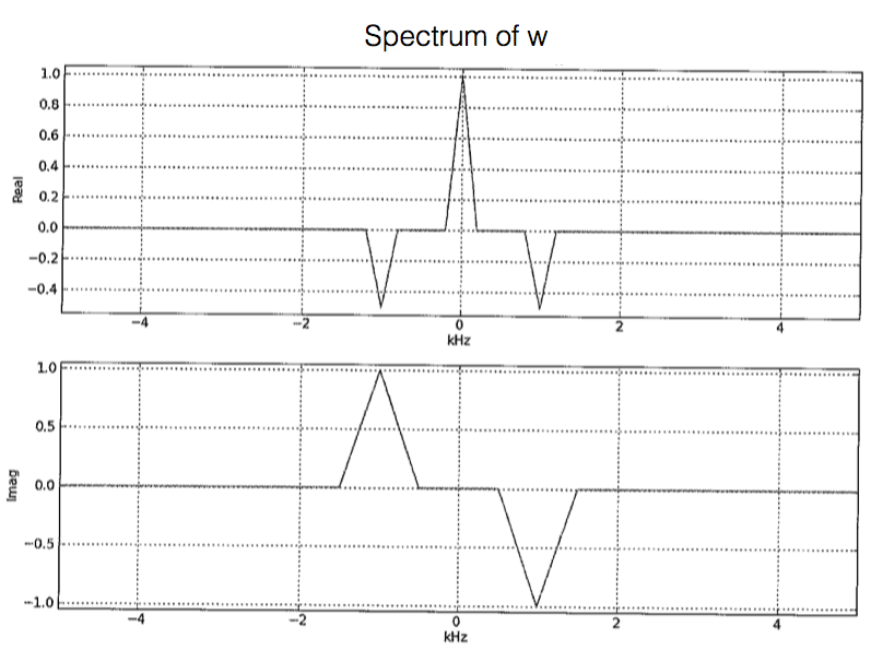
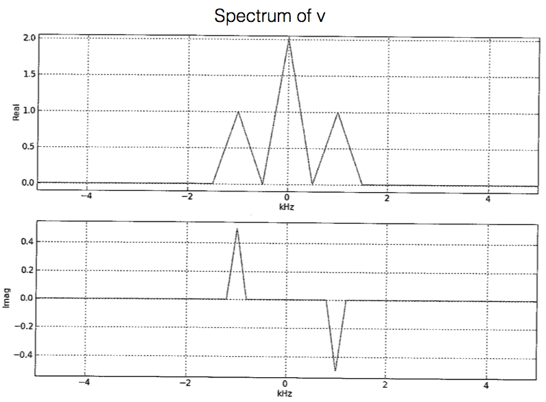
   Note that if $M=5$, the phase shift is $-\pi/2$, which produces $-\cos(...)$, which we can convert to $\cos(...)$ if the LPF has a gain of $-1$.