Quick Start Guide to Logic
Analyzers
(Gim Hom, gim@mit.edu)
Introduction
While
logic analyzers are similar to oscilloscopes, they differ in that logic
analyzer can have up to 136 channels of inputs to analyze and debug digital
systems. Oscilloscopes typically have a maximum of four inputs. The inputs to
the logic analyzer are attached to general purpose probes via “flying
leads”.
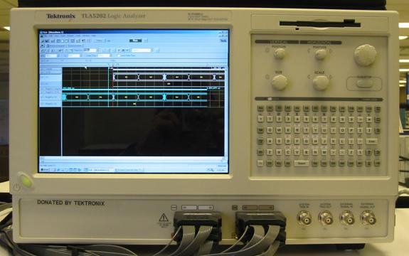
In
6.111 we will use a Tektronix TLA5202 Logic Analyzer (TLA) with 68 channels. The
Tektronix Logic Analyzer is a Windows 2000 based instrument. The instrument has USB ports that allow the
user to capture and store on to a USB drive anything that is displayed on the
screen. (PRINT SCREEN copies the entire
window display to the clipboard; ALT + PRINT SCREEN copies
the active window to the clipboard. You can use Windows program Paint or
Imaging to save the clipboard images.)
The
TLA samples at a 2 GHz rate. Under MagniVu, the TLA can burst sample at an 8 GHz (125 picoseconds)
rate. Keep in mind that the TLA stores the sampled data in memory. For a given
memory capacity, the total acquisition time decreases as the sample rate
increases. For example, if the memory holds 1 second of data when sampling at a
1 ms rate, it holds only 1 millisecond of data when the sample rate is
increased to 1 us.
Logic Analyzer Operation
There are four steps to
using the logic analyzer: connecting the leads, setting up the analyzer,
acquiring the data and analyzing the data.
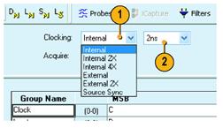
![Text Box: In setting up the analyzer, there are two types of data acquisition: internal clocking from the TLA or a signal from the unit under test. The clock can be the rising edge or trailing edge. Use the “Setup” window to select internal/external [1] and the sample rate (if internal) [2].](quick_la_files/image001.gif)
Data is acquired when a
triggering event occurs. Any of the following can be used as the trigger:
1. specific logic patterns or words
2. ranges: events that occur between a
low and high value
3. counter: a user programmed value
4. external signal
5. glitches
6. elapse time between two events or duration
of a single event.
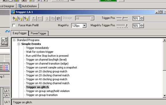
Use the “Trigger” window to
setup the triggering event.
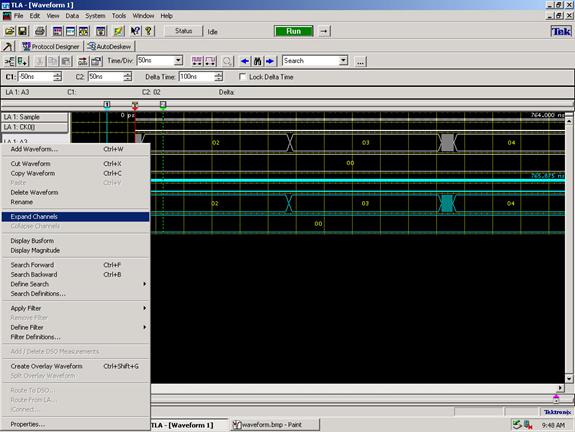
Once
captured, the data can be displayed in a many formats: hexadecimal, waveform
(collapsed or expanded with individual waveforms), and listing. Choose the
appropriate format for your application. For ease of analysis, the user can
rename each waveform (use right mouse click – rename). In addition, any combination of
channels can be grouped together in the display.
A TLA Tutorial – Measuring
the Glitch
- Power up the logic analyzer;
wait for it to boot into Windows 2000.
- Click on the program “TLA Application”.
You can use the wizard but it is easy and more useful to set up the TLA
without the wizard.
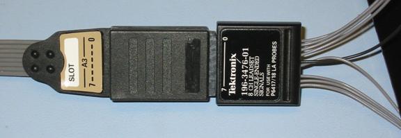
- Connect the “flying leads” to a
probe (default probe: A3). Signals should go to leads 0-7, and
ground to black. For the glitch measurement (Lab 1 - Exercise 3), attach
the clock to A3-0 and the glitch to A3-1. Note the orientation of the numbers
on the probe and the “flying leads’; they should match up.


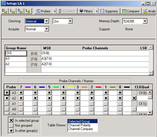
- Go the “Setup” window. Notice
that the clock is set by default to “Internal” at 2 ns. An external clock can be selected. You
can add additional probes if needed. CK0 separate line attached to the
probe cable and can be the external clock.
- Triggering: The TLA can trigger from a number of
trigger types. Use “Trigger immediately” for Lab 1 – Exercise 3 and
“Trigger on glitch” for Lab 1 – Exercise 5. To trigger on a glitch, find
the “Trigger” window and set the trigger event to “Trigger on glitch”
- Find the “Waveform” window. Click
“RUN” to start; alternatively, you can use the physical Run/Stop button in
the upper right hand corner of the TLA. Some students prefer to point and
click. Others prefer physical controls.
- Browse your data by moving the
sliders with the mouse, by changing “Time/Div”, and by using changing the
“C1” and “C2” parameters. Alternatively,
instead of using the mouse, you can use the control knobs in the upper
right hand corner of the instrument. “Scale” changes the “Time/Div”
setting. The large unmark control in
the upper most right hand corner of the front panel moves the selected
“slider” on the waveform window.
- Right-click on “LA1:A3” to expand and collapse signals.
Try to rename a waveform. You can
use attached keyboard or the keyboard on the instrument. Try to display
the signal in magnitude format.