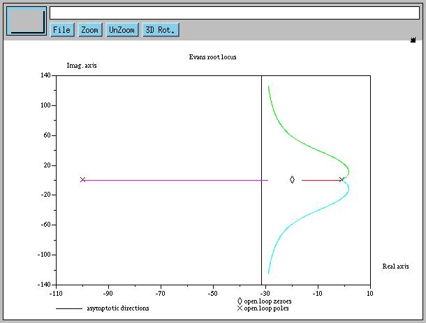
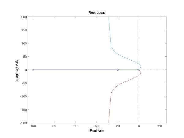
![[Graph not available because rendering was not complete even after several hours]](octave/rootLocus.jpeg)
This document describes how to perform common tasks in 6.302 using Octave, Scilab, and Matlab. The first two software packages are free alternatives to Matlab, and their use is encouraged.
Each software package employs different methods to create, examine, print, and save transfer functions. For the purposes of this tutorial, we will use the following transfer function as an example:
L(s) = 3e4 * (0.05s + 1)^2 / ((s+1)^3 * (0.01s + 1))
GNU Octave is a numerical computation software package very similar
to Matlab. In fact, the syntax is almost exactly the same. For help,
type help function_name. For an excellent
tutorial on control-related functions, type
DEMOcontrol.
For the purposes of 6.302, there exist two ways to create transfer
functions in Octave. The first is tf2sys, which takes as
arguments the coefficients of the numerator and denominator of the
transfer function. With the example transfer function, you would type:
L = tf2sys(3e4 * [0.0025 0.1 1], [0.01 1.03 3.03 3.01 1]);
Another command is zp2sys, which takes as arguments
the zeros, poles, and leading coefficient of the transfer function.
Consequently, you would type:
L = zp2sys([-20 -20], [-1 -1 -1 -100], 3e4);
You will notice that if you merely type L, the output
isn't very readable. Use sysout(L, "tf") to display the
function in polynomial form and sysout(L, "zp") for
zero-pole form.
For root locus, use rlocus(L).
L = tf2sys(3e4 * [0.0025 0.1 1], [0.01 1.03 3.03 3.01 1]);
title("Root locus of L");
rlocus(L);
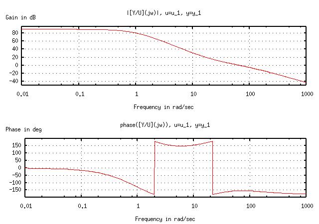
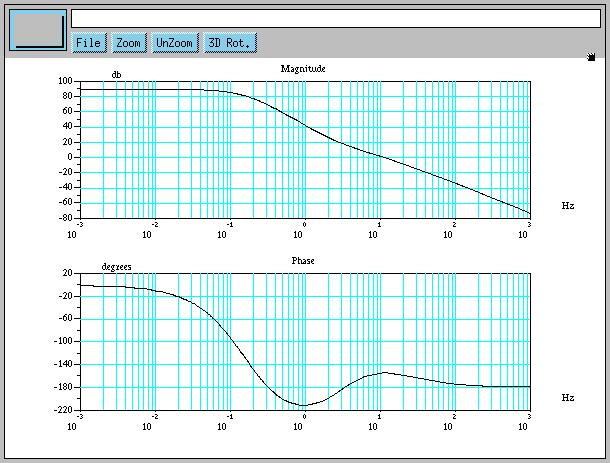
For Bode, use bode(L).
L = tf2sys(3e4 * [0.0025 0.1 1], [0.01 1.03 3.03 3.01 1]);
bode(L);
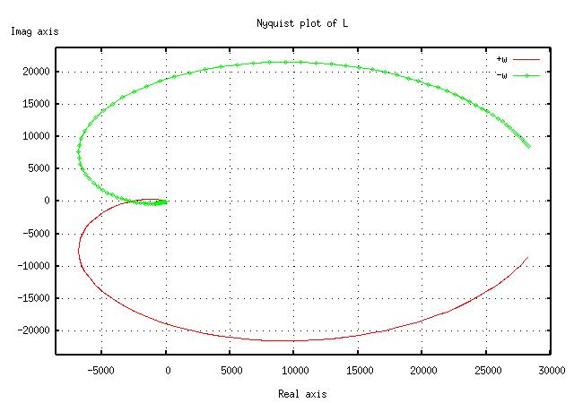
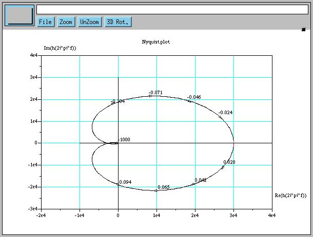
For Nyquist, use nyquist(L).
L = tf2sys(3e4 * [0.0025 0.1 1], [0.01 1.03 3.03 3.01 1]);
nyquist(L, logspace(-1, 1, 100));
title("Nyquist plot of L");
xlabel("Real axis");
ylabel("Imag axis");
replot;
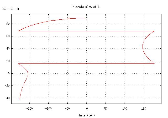
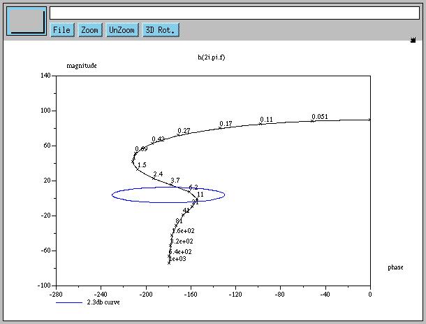
For Nichols, use nichols(L).
L = tf2sys(3e4 * [0.0025 0.1 1], [0.01 1.03 3.03 3.01 1]);
nichols(L);
title("Nichols plot of L");
replot;
As in Matlab, the commands title, xlabel,
and ylabel assign strings to the graphs. Often after
these commands, replot is necessary to activate the changes.
However, bode does not work after a replot
command; if you find yourself in a situation where a replot
is necessary, plot the data from bode manually using
plot. (See the online help for details.)
Octave uses Gnuplot to plot its graphs, so the saving and printing process is not as straightforward as clicking a button.
To save a graph in PNG format (which can be read by almost any graphics program), use the following commands:
gset terminal png;
gset output "filename.png";
replot;
Again, with Bode plots, just use bode(L) again instead
of replot.
To print a graph, use the following commands:
gset terminal postscript;
gset output "|lpr";
replot;
After saving or printing, reset the environment with the command
gset terminal x11, or else any subsequent graphs will be
saved/printed without being displayed onscreen.
Scilab is a free software package similar to Maple. Its syntax is considerably different from Matlab, but Scilab can perform symbolic manipulation, unlike Matlab. It includes excellent demos, as found by pressing the "Demos" button on the toolbar.
This is perhaps the easiest task of all. Just type the following:
s = poly(0, "s");
L = syslin('c', 3e4 * (0.05*s + 1)^2 / ((s+1)^3 * (0.01*s + 1)));
The poly command simply defines a polynomial with the
symbol "s." Don't forget it! Simply type L to see the
transfer function you've just defined.
For root locus, use evans(L).
s = poly(0, "s");
L = syslin('c', 3e4 * (0.05*s + 1)^2 / ((s+1)^3 * (0.01*s + 1)));
evans(L, 2.6);
For Bode, use bode(L).
s = poly(0, "s");
L = syslin('c', 3e4 * (0.05*s + 1)^2 / ((s+1)^3 * (0.01*s + 1)));
bode(L);
For Nyquist, use nyquist(L).
s = poly(0, "s");
L = syslin('c', 3e4 * (0.05*s + 1)^2 / ((s+1)^3 * (0.01*s + 1)));
nyquist(L);
For Nichols, use black(L).
s = poly(0, "s");
L = syslin('c', 3e4 * (0.05*s + 1)^2 / ((s+1)^3 * (0.01*s + 1)));
black(L);
Unfortunately, there doesn't seem to be any easy way to replace
pre-existing titles and axis labels. If you want true customization,
consider using plot2d manually.
Just use the menu items on the graph screens.
Matlab is one of the de facto standards of scientific computing. Though it is very powerful, it is unfortunately also very expensive. This is why the availability of packages like Octave and Scilab is so desirable. Nevertheless, the following Matlab material is provided for reference and comparison.
Like Scilab, Matlab makes this relatively easy. Just type the following:
s = tf ('s');
L = 3e4 * (0.05*s + 1)^2 / ((s+1)^3 * (0.01*s + 1));
For root locus, use rlocus(L).
s = tf ('s');
L = 3e4 * (0.05*s + 1)^2 / ((s+1)^3 * (0.01*s + 1));
rlocus(L);
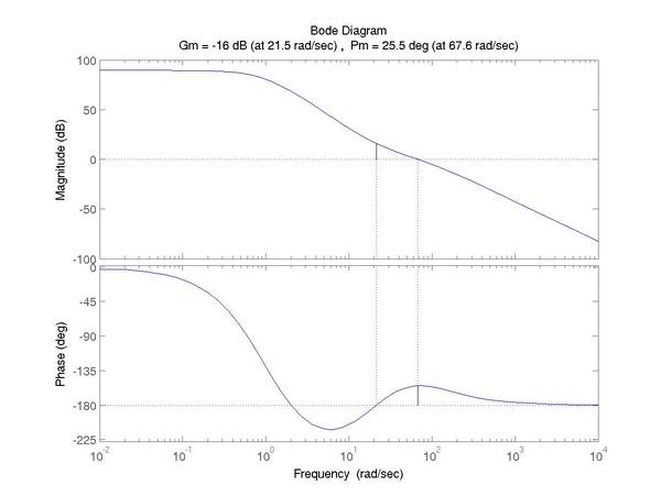
For bode, with margins displayed, use margin(L).
s = tf ('s');
L = 3e4 * (0.05*s + 1)^2 / ((s+1)^3 * (0.01*s + 1));
margin(L);
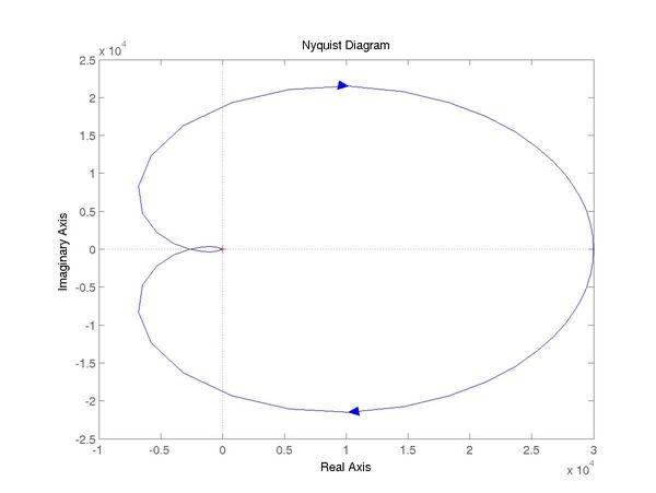
For Nyquist, use nyquist(L).
s = tf ('s');
L = 3e4 * (0.05*s + 1)^2 / ((s+1)^3 * (0.01*s + 1));
nyquist(L);
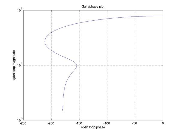
For Nichols, you must calculate the magnitude and phase separately
with nichols(L), then explicitly graph it (probably as
a semilog plot).
s = tf ('s');
L = 3e4 * (0.05*s + 1)^2 / ((s+1)^3 * (0.01*s + 1));
[m,p,w] = nichols(L);
semilogy (p(:,:), m(:,:));
grid;
title ('Gain/phase plot');
xlabel ('open loop phase (deg)');
ylabel ('open loop magnitude');
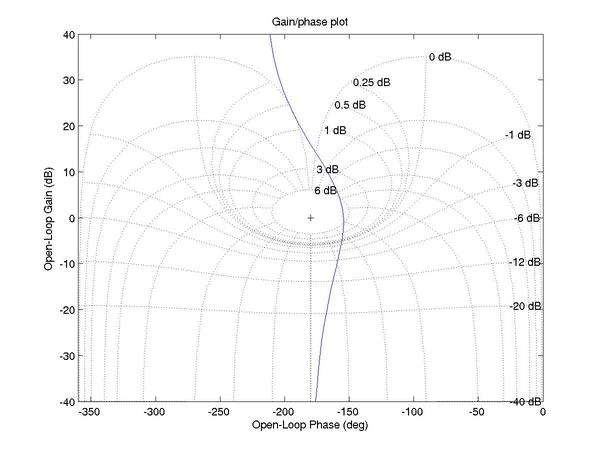
You can also show the Nichols Chart on a dB axis:
s = tf ('s');
L = 3e4 * (0.05*s + 1)^2 / ((s+1)^3 * (0.01*s + 1));
[m,p,w] = nichols(L);
plot (p(:,:), 20*log10 (m(:,:)));
ngrid;
title ('Gain/phase plot');
xlabel ('Open loop Phase (deg)');
ylabel ('Open loop Magnitude (dB)');
Again like Scilab, Matlab provides a menu interface that makes it easy to save and print graphs as needed.