Massachusetts Institute of Technology
6.877 Computational Evolutionary Biology, Fall, 2007
Laboratory 2, Part I: Evolution, polymorphism, and the coalescent
Handed out: November 12, 2007 Due: November 21, 2007
This portion of the laboratory is PART I of 2 parts. PART II will be handed out at the end
of this week. PART I consists of a
series of ‘problem set’ type exercises followed by some warmup computer exercises,
covering the material from chapters 2 and 3 of Gillespie. In addition, there is
are two group questions (questions 11 and 12, the last 2 in this part)
that I’d like you to solve and then bring to class for discussion next Monday.
Preamable: some review and ‘cheat sheet’ summary.
In preparation, please read, or re-read, chapter 2 of
the Gillespie text, as well as the pages in the Rice text mentioned below.
0. Definitions and descriptive statistics for DNA
sequences
Heterozygosity (also known as
‘gene diversity’) is the probability that
two random DNA (or gene) sequences
are different. To calculate it,
one can straightforwardly examine all sequence pairs and count the fraction of
the pairs in which the two sequences are different from each other. It is often faster to start by counting
the number of copies of each type in the data. Let ni denote the number of copies
of type i and let n be the sum of all these types. Then heterozyosity is estimated by:
![]()
You may recall that Gillespie,
page 27, eqn. 2.3, gives a formula for the decay of heterozygosity (genetic variation or variance) via
drift, generation by generation.
Gillespie p. 30, eqn. 2.10, gives the fundamental formula for the
equilibrium value of heterozygosity at mutation-drift balance. Equation 2.10 introduces the important
‘combined’ parameter commonly denoted by theta, q, which is equal to 4Nu, where u is the mutation
rate, and N is the population
size. (We’ll make that the ‘effective’ population size just below). This parameter q is
of crucial importance in studying evolution at the gene level and
determining the relative ‘power’ of selection vs. migration vs. drift with
respect to population size.
Number of segregating sites. A
‘segregating site’ is a site that is polymorphic in the data, i.e., it shows up
as distinct gene types, or alleles.
The number of segregating sites is usually denoted S (or Sn if referring to n samples).
Mean pairwise difference. Let kij
denote the number of nucleotide site differences between sequences of type i and sequences of type j. The mean pairwise difference is:
![]()
Mean
pairwise difference per nucleotide. If the
sequences are L bases long, we can standardize the above value by
the length of the DNA sequence:
![]()
A second formula for this calculation is given by Gillespie on page
44, equation 2.16, and the following equation on page 45.
Mismatch distribution. A
histogram whose ith entry is the number of pairs of sequences that differ by i sites. Here i ranges from 0 through the maximal difference between pairs in the
sample.
Site frequency spectrum. A
histogram whose ith entry is the number of polymorphic
sites at which the mutant allele is present in i copies within the sample.
Here, the indexing i ranges
from 1 to n–1.
Folded site frequency spectrum. Often
one cannot tell which allele is the mutant and which is ancestral. In that case, we combine the entries
for i and n–i so the
new i ranges from 1 through n/2.
Neutral substitutions. The
rate at which neutral (non selected) mutants are substituted into the
population.
The number of new mutant genes introduced per generation. In a population of 2N genes, i.e., the
diploid case, this number is 2Nu.
The fraction of those mutants that eventually become fixed. If drift continues long enough, all but one of the
genes in the current population will be lost, and the one that survives will be
fixed. Each gene has a probability of 1/(2N) of increasing to
fixation (its initial frequency).
Neutral theory.
The rate of substitution is the
number of new mutants per generation (2Nu)
times the probability that a given mutant will be fixed, 1/(2N). So
the product of the two is just u:
remarkably, the substitution rate is just equal to the rate of mutation of
neutral alleles. (See equation
2.12 of Gillespie). It does not
depend on the size of the population or the extent of subdivision within it.
We now turn to the problem set questions.
Question 1. Effective population size.
The effective
population size, Ne, plays a
crucial role in all the theoretical accounts of evolution. Effective population size is to be
distinguished from the census population size (the actual count of
individuals in a population). Since we multiply this (typically large) Ne number by another (typically very small) factor, s,
u, m, or r (recombination
rate), to get the crucial value of theta, it’s important to get this value as
correct as we can make it, because this will have profound impact on the
outcome of polymorphism patterns. Thus, it’s actually extremely important to
figure out how to correct for different variations that are actually seen
biologically. Gillespie section 2.7, pp. 47 on, shows how to
correct for fluctuating population size by ‘back calculating’ what the
population ‘should have been’ in order to get the same change in variance as
would be produced by a ‘pure’ Wright-Fisher model. This idea, viewed from
another perspective, is also covered in the Rice book, pages
111–112. Here’s another
common correction that is often encountered in biological situations.
Elephant seals possess an
interesting system of mating. One
alpha-male lies in the center of a harem of females and attempts to mate with
as many of these females as possible throughout the course of the mating season. The harem is also surrounded by 5
beta-males, usually younger and smaller, who lie around the harem and protect
it from invasion by other males.
When the alpha-male starts to mate, the beta-males use his distraction
to do some mating of their own with the females at the outer edges of the
harem. Other males, not alphas or
betas, stay in the water and are not allowed to mate at all. One would think that the alpha male
sires the most offspring in this situation, however, recent genetic studies
have found that beta-males as a group actually have at least as much mating
success as the alpha-male. From a
typical harem 50% of the children are sired from beta males and 50% are sired
from the alpha. Given that there
are 40 alpha-males, and 2000 females in the population, assuming that each of
the harems is exactly the same size, assuming that all beta-males have exactly
the same probability of having an offspring, and assuming that all females are
fertile and available for mating, calculate the effective population size for this population of elephant seals. NOTE: assume non-overlapping
generations for simplicity.
To
solve this problem, you should read the relevant section in the Rice textbook,
pages 113–114; please show
the details of your work and how you arrive at your answer (not just a final number!) (And, Yes, one can just go through the
Rice book and follow that derivation, but it’s more interesting to work out the
details as applied to this particular case.)
Question 2. Neutral evolution
and drift. How would an increase in population size affect the rate of
neutral substitutions in the generations immediately following the increase?
Question 3. Neutral evolution
and drift. Consider a stretch of noncoding, nonfunctional DNA
that is 1,000 nucleotides long. We
can thus assume that it is not under selection – it evolves
neutrally. Assume that the mutation rate is high – 2 changes per site per
million generations.
Question 3(i) In a
population of 10,000 individuals, how many new alleles will be created in the
population each generation?
Question 3(ii) What
fraction of these new alleles will ultimately be fixed?
Question 3(iii) What
is the rate of molecular evolution? (substitutions per site per generation)
Question 3(iv) In a population of 50 individuals with the same
mutation rate, how many new alleles will be created per generation? What fraction of these will ultimately
be fixed? What is the rate of
molecular evolution?
Question 3(v) Which
population will have greater heterozygosity at any one time? Why?
Question 4. The neutral theory of evolution
Question 4(i) In a population of 10,000 individuals with a
neutral mutation rate of 1 nucleotide change per site per 10 million
generations, what is the expected heterozygosity per site?
Question 4(ii) What is the expected heterozygosity for a protein
that is 500 amino acids long?
Express the meaning of this result in a sentence (i.e., express it in
words).
Question 4(iii) What is the expected heterozygosity if there are 12
individuals in the population?
Question 5. Segregating sites,
S.
What is the ratio between the expected
value of S in a sample of 100 DNA
sequences and the expected value in a sample of 200? (You should do the
calculation, and, if you want to go a little further, try to derive the ratio
mathematically). See equation 2.14 of Gillespie for more details.
Question 5. Nucleotide polymorphisms and the number
of segregating sites, S
Here is a set of 10 (real) DNA
sequences, each with 40 sites, taken from a mitochondrial DNA sample:
seq1 AATATGGCAC
CTCCCAACCC TCTAGCATAT ACCACTTACA
seq2 .......T..
.C......TG C......C.. ..........
seq3 ..C.......
.......... .......... ..........
seq4 .......T..
.C......TG C......... G.........
seq5 ..........
.......... .......... ..........
seq6 .....A....
........T. C......... G....C....
seq7 ..C....T..
.C......TG C......... G.........
seq8 .....A.T..
TC......TG C......... G.........
seq9 ..........
.......... C......... ..........
seq10 .G...A....
........T. C......C.. .T....C..G
Each column corresponds to a different site. Periods indicate sites that are
identical to the site in sequence 1.
To save typing, the file is available for download here: Question 5 sequence data.
Use these data to answer the following questions.
Question 5(i). Calculate the mean pairwise difference among the sequences,
the nucleotide diversity p.
(See p. 45, and equation 2.13 of Gillespie.)
Question 5(ii). Use this value to estimate q.
Question 5(iii). Calculate the number of segregating
sites, S, directly from the data sample (more properly denoted S10).
Question 5(iv). Use
this value to provide a second estimate of q,
using equation 2.15 of Gillespie.
This is known as the Waterston segregating sites statistic; it is
based on coalescent theory.
Question 5(v). What
might you infer from the similarity (or dissimilarity) of these two estimates?
To ease your task a bit here, I
have posted a very simple awk script piS that computes the diversity statistic p and
an estimate of q
based on the Waterston segregating sites statistic (along with some other
things, viz, Tajima’s D statistic), for
a set of aligned sequences like this.
The script is available here, and ought to run
(i.e., it’s been tested on) any linux box; Mac OS X, etc. (you can download it as a text file and
run it locally – I will check re getting it going on Athena if need be). It is invoked this way:
awk –f piS.awk <name of sequence file>
> <myhomedir>myoutputfile.txt
where you should make sure myoutputfile.txt is a file in your home directory. Running this program should give you output like the following (not these results – this is from a different data set!)
pi: 53.626812
Segregating
sites: 184/1878
theta_hat[estimated from
S]: 49.273068
Tajima's D: 0.354335
a1=3.734292 a2=1.602387
b1=0.362319 b2=0.242754
c1=0.094530 c2=0.067558
e1=0.025314 e2=0.004345
The a1, a2, etc. coefficients are those needed to compute Tajima’s D, as part of the variance calculation devised by Tajima. This is a method to detect the ‘fingerprint’ of selection that we shall cover later on.
Question 6. (Coalescent
theory.) Four genes can have two possible
different unlabelled coalescent trees.
Sketch the two trees and work out the respective probabilities of their
occurrence.
Question 7. (Coalescent
theory; probability theory required – extra credit).
In a coalescent tree of three
genes let T3 , T2 be the times respectively while there are three and
two ancestors of the genes. Derive a formula time to the most recent common
ancestor W = T3+T2.
Questions 8 and 9
(Coalescent theory simulations)
If you want to cut to the
chase and get to the actual questions, they are a few pages on, labeled
“Questions”, but I would urge that you try out the ms program as suggested below.
Warm-up using simple coalescent computer programs
There are three or four readily available computer programs that are used to work with coalescent analysis in conjunction with polymorphism data. There is a java applet simulator for some very simple coalescent simulations, available at http://www.coalescent.dk/. Several other programs take the trees produced by these programs and then generate ‘artificial’ sequence data sets by sprinkling in Poisson-distributed mutations. In typical ‘simulation’ mode, given polymorphism data like the one you saw in the earlier sections of this lab, one can use the coalescent to simulate possible polymorphism pattern outcomes, and thus derive predicted polymorphism patterns, given various scenarios of population size changes, recombination, etc., all using basic parameters derived from the original data. We can then go back see which scenario is most compatible with the data – in the stronger sense of also obtaining confidence intervals for some of the test statistics we have seen above. (These might be otherwise quite hard to derive.)
Another mode is rather different:
instead of exploring the parameter space ‘by hand’ we can use likelihood
methods to try to find the ‘best’ estimates for effective population
size, mutation rate, and so forth.
In this part of the lab, we shall deal only with the former, ‘hand simulation’ method to just ‘get acquainted’ with how to run a coalescent program and use it to simulate a set of sequences.
In particular, we will use
Hudson’s computer program ms, which
simulates coalescent gene trees under a variety of possible population change,
migration, recombination, and other historical scenarios. We use this program mostly because it
is fast and accurate and can compile on almost any platform with a decent C
compiler. Instructions for
installing it are given below.
Installing and running the ms program.
To get going, you’ll have to
download the ms.tar
file from Hudson’s site here. Un’tarring will give you a directory msdir that contains
both the pdf documentation and all the source files you need. You simply cd to this new directory and
then compile three programs, ms,
stats, and sample_stats:
gcc –O3 –o ms ms.c
streec.c rand1.c -lm
gcc
–o stats stats.c -lm
gcc –o sample_stats
sample_stats.c tajd.c -lm
See the README file distributed
in msdir for further details.
Here I’ve chosen a particular random number generator – I suggest you use
this one so your results will ‘agree,’ with other folks, but see the ms documentation about the choices
(it’s not really of concern here ).
Using the ms program.
A complete pdf documentation file
is located here. (and in the msdir directory). Running the program
with ms –h
will produce a summary of all the command line arguments. As the documentation itself says:
In its most basic mode, the user supplies a command line in the form:
ms nsam nreps -t θ
The above line shows the
simplest usage of ms that
generates samples under the basic neutral model, with constant population size,
no recombination, panmixis (free interbreeding), and an infinite-sites model.
In this case there are three arguments to ms:
nsam, nreps, and,
following the switch “-t”, the
parameter θ. The two arguments, nsam and nreps are required and must appear in this
order.(Although there are
exceptions, most of the switches can appear in any order.) nsam is the number of copies of the locus in each sample, and nreps is the number of independent samples to generate. The third parameter here is the mutation
parameter, θ = (4N0μ) where N0 is the diploid population size and where μ
is the neutral mutation rate for the entire locus. Remember that for
most purposes, this basic parameter is ‘small’, between 0 and, say, 20! At
least one of the options, -t –s,
or -T must be used. The
latter two options are described later. After nsam and nreps, any or all other switches with their
parameters can be read from a file using -f filename.
Example:
ms 4 2 -t 5.0
In this case, the program will
output 2 samples, each consisting of 4 chromosomes (or ‘sequences’),
generated assuming that θ = 5.0.
The output from the example
command in the previous section would look like this (the exact output will
depend on the random number generator) :
ms 4 2 -t 5.0
27473 36154 10290
//
segsites: 4
positions: 0.0110 0.0765 0.6557 0.7571
0010
0100
0000
1001
//
segsites: 5
positions: 0.0491 0.2443 0.2923 0.5984 0.8312
00001
00000
00010
11110
Here’s how to intepret the
output. The first line of the output is the command line. The second line shows
the random number seeds. Following
these two lines are a set of lines for each sample. Each sample is preceded by
a line with just “//” on it. That line is followed by “segsites:” then the
number of polymorphic sites in the sample. Following that line is a line that
begins with “positions:” which is followed by the positions of each polymorphic
site, on a scale of (0,1). The positions are randomly and independently
assigned from a uniform distribution. (With recombination, the distribution is
somewhat more complex.) Following the positions, the haplotypes (sequence
blocks) for each of the samples is given, as a string of 0’s and 1’s. The zeroes denote the ‘ancestral form’,
while the ones denote the mutant or ‘derived state’. (Recall that the infinite sites
model only admits a binary change at any one site position.) A sample line is omitted if there are
no mutations from the initial state of all zeroes.
ms nsam nreps -T
When the option -T is used the trees representing the
history of the sampled chromosomes are output. For example, the command line ms 5 2 -T results in the following
output:
ms
5 2 -T
3579
27011 59243
//
((2:0.074,5:0.074):0.296,(1:0.311,(3:0.123,4:0.123):0.187):0.060);
//
(2:1.766,(4:0.505,(3:0.222,(1:0.163,5:0.163):0.059):0.283):1.261);
This output represents the
trees for two samples. The tree format is in a commonly accepted particular
list form that we’ll study more closely when we look at phylogenetics in the
latter part of the course. This
particular list form is called Newick format, and is used by the Phylip
phylogenetic program and a number of other applications. The branch lengths are
in units of 4N0 generations. The sampled
chromosomes are labeled 1, 2, ..., corresponding to ordered, sampled
chromosomes. This labeling is irrelevant for unstructured population models,
but with island models described later, the labeling can be important. With recombination a tree is output for
each segment within which no recombination has occurred in the history of the
sample.
ms 5 10 -t 6.0 | grep segsites | cut -f 2 -d ’ ’ >
SegSites.txt
Questions
Now we can test some theory.
Let’s use coalescent simulations to estimate the average number of segregating
sites when n = 5, and theta
= 6.0, by generating 10,000 replicate samples, using unix to snip out the
segregating sites from the output, and passing that to a simple statistical
analysis program that is also in the same package. Selecting out the second column via the ‘cut’ command will
give us just the mean value and the standard deviation:
ms 5 10000 -t 6.0 | grep segsites | cut -f 2 -d ’ ’ |
stats
Remember Watterson found
analytically that the expected number of segregating sites ought to be as
follows (as in Gillespie, equation 2.15):
![]()
Question 8.
Work out what the expected value
should be for n=5 and this particular
value of theta. Then compare the
theoretical result to what you get via the simulation – please provide both answers.
How much closer does your
estimated value come to the true value of theta as you increase the number
replicates by one and then two orders of magnitude?
Note that the stats program will also print out and
particular percentile statistic for the data on a particular column fed into
it, including the median and, say, the 99th percentile of the distribution,
via this form:
stats 0.5 0.99
Thus, you could actually use
the output from this program to feed a graphing program to view the
distribution of any quantity of interest (see the next paragraph below, e.g.).
For other sample statistics,
including Tajima’s D, we can use the sample_stats program
by Hudson in the same package. The
program will compute the nucleotide diversity p, the number of
segregating sites, Tajima’s D, and
two additional statistics we haven’t yet discussed.
ms
30 4 -t 3.0 | sample_stats
pi: 1.751724 ss: 6 D: 0.446936
thetaH: 1.282759H: 0.468966
pi:
1.705747 ss: 9 D:-0.774289 thetaH: 0.501149H: 1.204598
pi:
1.390805 ss: 6 D:-0.233099 thetaH: 1.022989H: 0.367816
pi:
3.156322 ss:15 D:-0.560417 thetaH: 3.119540H: 0.036782
Question 9.
Now you can use these three
programs piped together to show that, say, for n=5, q=6.0, E[p]=q, as
expected by theory. Try this by
generation 10,000 replicates with these values: first generate the samples
using ms, then pipe these through sample_stats; then pull the 2nd
column from this output and feed it to stats. (You can use the unix ‘cut’ program
as before, via cut –f 2 to pull
out the 2nd column from the output of sample_stats
and thus get the mean value of p.)
Question 9(i) Please do this for several different replicate sizes
and provide a table of E[p], q, and indicate how close the convergence
is.
Question 9(ii) Because individuals are correlated through their
common ancestry, increasing the number of individuals does not lead to
proportional increases in the performance of an estimate. Theory predicts that
as the sample size becomes infinite the standard deviation of our estimate of q
(based on nucleotide diversity) will be as follows:
![]()
Using ms and
the program pipeline as above, please test the theoretical predictions against
simulation for q=4.0. First, compute the theoretical
limit. You might want to use,
e.g., 10,000 simulated samples at a time, while increasing n and then plot the resulting standard deviation
against n, in gnuplot, or Excel,
Matlab, etc. also indicating where the theoretical limit is. Here’s the sample output you might get
for q=1.0.
TrueTheta n MeanEstimate SDEstimate
1 2
0.979800 1.372655
1 3 0.984733 1.093850
1 4
1.006700 0.993173
1 5
1.005380 0.940195
…
1 12
0.989418 0.802780
1 13
0.998744 0.808657
1 14
0.991237 0.791793
1 15
1.001560 0.811949
Question 9(iii) Briefly comment on the implications of your results
for sequence sample collection.
Questions 10 and 11 [in
class problem solving.]
OK, for the last question
– a change of pace:
Please work these problems in
a a group and come to class next Monday, Nov. 19th prepared to go through
your reasoning. You’ll have to recall the formulas for Sn, p, the neutral mutation
equation, the formulas for selection, and so forth, and put them together in
creative ways. In addition,
these problems require two additional bits of theory, which are described afterwards:
(1) the (Jukes-Cantor) ‘correction’ for multiple nucleotide substitutions; and
(2) the change in effective population size resulting from the
mutation-selection balance. We
will present them here with a minimum of explanation, reserving details for next
Monday. Please come prepared to discuss!
Question 10. You
are studying a neutral, unconstrained (i.e., neutral, no selection) region on a
non-recombining chromosome in two species of butterflies. You know that this neutral region is
linked to a region that contains 100 genes each of the length 1kb. Each of
these 100 genes is constrained to the same extent.
To understand the pattern of
background selection, you sequence 1 kb from the unconstrained region and 1kb
from a constrained (i.e., non-neutral)
gene region in both species. You find that the unconstrained region differs at
247 sites between the two species and the constrained region differs at 94
sites.
You also sequence 2 alleles
different by origin of 1 kb long in the unconstrained region and find that you
have 4 differences. For comparison you sequence 2 alleles different by origin
of 1kb each from a neutral region about which you know for a fact that it is
unlinked to any constrained regions. In those 2 alleles you find 80
differences.
Assume that neutral theory holds
for the distribution of selection coefficients of new mutations. Assume further
that deleterious mutations are codominant (selection heterozygosity factor h=
0.5), that selection acts on each independently of the others, and that they
all have the same selection effect.
Also, assume that these butterflies go through 5 generations per year
and that they last shared common ancestor 10 million years ago.
(1) What is the Ne of the species of butterflies from which
you drew the polymorphism data?
(2) What is the rate of
deleterious mutations occurring per any one of the constrained genes per
generation?
(3) What is the selection
coefficient s of the deleterious
mutations at the constrained region?
(4) Is the selection coefficient
you find consistent with your assumption that these mutations are strongly
deleterious? Explain.
(5) You learn that in the other
species of butterflies (the one in which you have not yet collected any
polymorphism data) there is a translocation of 100 more genes to the
nonrecombining chromosome, such that the same unconstrained region on that
chromosome is now linked to a region containing 200 constrained genes. What is
the length of the unconstrained region that you need to sequence such that you
would expect to find (about) 1 segregating site in comparison of 11 sampled
alleles (i.e., the sample size n=11)?
Question
11. Orcs and goblins are two related evil species in the Middle Earth. They
had a common ancestor 20 million years ago. For the first 10 million years both
lineages had the same mutation rate and the same generation time (1 generation
per 20 years). Then for an unknown, but undoubtedly magical and thoroughly evil
reason orcs evolved a 2-fold higher mutation rate per generation and goblins
evolved a faster generation time (1 generation per 10 years). Consider two
neutral regions A and B of identical length. Region A is linked to a highly
constrained gene X. Region B is unlinked from A and X and is not linked to any other constrained
region. Assume for simplicity that only neutral and deleterious mutations
happen in X.
(1) Suppose
you compute a ‘relative rates test’ in the region A. That simply means
computing the mutation rate per generation times the total number of
generations since the split between orcs and goblins. Would you expect to detect a difference in the rates of
evolution in the orc and goblin
lineages? Region B? Explain your answers.
(2) Assume
that goblins and orcs currently have identical effective population sizes. You
sample the same number of alleles in the regions A and B in both orcs and
goblins. You discover that in goblins there are 3 times fewer segregating sites
in A than in B. What is the expected ratio in the numbers of segregating sites
in A and B in orcs? [Hint: one can also look at the ‘effective population size’
relative to a region as well as for an entire population.
(3) Now
suppose that you know specifically that orcs have a small effective population
size of Ne = 10,000, because
of frequent bottlenecks. You sample 20 alleles length 1000 bp of the region A
and identify 40 segregating sites. What is your estimate of the proportion of
differences that you expect to see between regions A sampled in orcs and
goblins?
To solve
both of these questions you will need to review Gillesipie, chapter 2. Plus:
Two additional pieces of theory...
(1) The
(Jukes-Cantor) ‘correction factor’ for observed vs. ‘actual’ number of
nucleotide differences.
So far we have done our
computations on polymorphism sequences based on just the observed counts, all
on the assumption that we were looking at individuals from the same
species. However, when we look
across species, or even within species, if the time since common divergence is
long enough, there is always the possibility that the same nucleotide site
position could have changed more than once. For example, position 1, say, could first be an A; then be
substituted with a T; and then once more back to A. In this case, we would not ‘see’ any change from the
ancestral state even though a change had occurred. We call this a ‘multiple hit’. (So in a way this relaxes the constraint of the infinite
sites model.)
In general then, the number of
nucleotide substitutions that we observe, and that we have been calling
mutations, are always an undercount of the true number. There are many models of nucleotide
substitutions that have been proposed to provide a ‘correction factor’ for this
possibility, and we will explore these more thoroughly, but for these problems
you can rely just on the simplest, the Jukes-Cantor (1969) formula.
Here is the correction
equation. Suppose we look at L sites in two nucleotide sequences and find that they
differ by an observed proportion D. (E.g., if two sequences are 1000bp long and differ in 10 positions,
then D=10/1000=0.01. The actual expected proportion
of sites different is given by the following correction:
![]()
So for example, in our case, we
would have K=3/4
ln(1–4/3x0.01)=0.01006 proportion (not much of an undercount in this
case). Note that we could also
apply the correction to actual counts, rather than proportions.
The Jukes-Cantor correction is
based on a very simple Markov chain model stating that each nucleotide base A,
T, G, C has the same probability at every step of changing into any of the
other three bases, at rate a, and a rate
1–3a of staying the
same. This forms a transition
matrix. If one goes through the math of this Markov process, as we shall do in
class, one will find that the possible divergence leads to the stated
correction formula. This model is
clearly unrealistic, in that the actual transition probabilities from one base
to another are not equal, and, in fact, in this model, lead to a long-term
steady state distribution of probabilities of each nucleotide of ¼ (as
might be expected from the symmetry of the model).
(2) The change in effective
population size due to the mutation/selection balance in the case of
deleterious alleles.
So why is
variation lower in the two regions? The presumed answer is that natural
selection is removing deleterious mutations as these ‘bad’ mutations are
‘dripping in’ at some rate during each generation at the linked locus, a
process that is sometimes called background selection. This idea was advanced by Brian
Charlesworth (1993) as one way to explain the reduced variation that Kreitman
found in his Drosophila data. (Reference: Charlesworth, B., et al 1993. “The effect of deleterious mutations on neutral
molecular variation,” Genetics
134:1289–1303.
If there is ‘background
selection’ against deleterious genes, then one’s intuition is that by getting
rid of these genes (and so individuals), the population size might be a bit
reduced. We can quantify this
intuition, in a way that leads to a formula that will also be of use when we
talk about the accumulation and elimination of deleterious alleles. In general, we would like to derive the
frequency of the classes of individuals with i mutations, which are assumed to be deleterious. (If i=0, then this is the case of zero deleterious
mutations.) We will use this later
on in the discussion of a model of
the accumulation of deleterious mutations known as “Muller’s ratchet” –
an effect where deleterious mutations accumulate on a chromosome faster than
selection can get rid of them (until the species goes extinct!). Muller proposed that one
explanation for the existence of
sexual reproduction was that it could remove this possibility. Gillespie explores this model on pp.
174-178, and we follow his exposition below.
We shall state only the result
first. This basically tracks through what happens if we assume that mutations
are Poisson distributed, then uses that to find the frequency of individuals
after reproduction; then applies the change due to selection, in the usual way,
using the equation that includes the selection coefficient s and the heterozygote advantage coefficient h.
The frequency of individuals with
i (deleterious) mutations at
selection-mutation equilibrium, given mutation rate m,
selection coefficient s, and
heterozygous advantage factor h
is given by the following Poisson distributioin:

We can plug in i=0 to
get the equilibrium frequency for 0 deleterious mutations.
In more detail, following
Gillespie, we have the following.
To get the basic model here, we
follow what is sketched out in Gillespie, pp. 174-178. Here is his derivation
of the reduction in effective population (actually ‘allele number’) size due to
background selection, based on the calculation of the frequency of alleles with
a particular number of deleterious alleles. It is an exercise in the addition of Poisson distributions
(which are also Poisson). Besides
its use in the background selection formula, this is part of an intriguing
model about the power of (sexual recombination) to eliminate deleterious
mutations. Otherwise, if selection
cannot get rid of such mutations faster than they accumulate, the number of
mutations will increase monotonically, a phenomenon known as Muller’s ratchet
(after the theorist who proposed it).
So let’s give a brief presentation of Muller’s ratchet and then give the
derivation for the effective population size reduction.
Muller’s ratchet.
Assume a population N of asexual (but diploid)
individuals. Each individual will have a certain number of deleterious
mutations sprinkled on its chromosomes. Assume that the mutation rate to
deleterious alleles at any particular locus is so small that all deleterious
mutations are heterozygous with the normal allele. Individuals may be grouped
with respect to the number of deleterious mutations they possess. A fraction x0 of individuals will have no deleterious mutations, a
fraction x1 will have
1 deleterious mutation, and so on. If the number of individuals with no
mutations, Nx0 is
small, then this class will be subject to genetic drift. Should drift cause the
loss of all individuals with no mutations, then each individual in the
population will have at least one deleterious mutation, and Muller’s ratchet
will have clicked once. If the number of individuals with one mutation, Nx1 is small, then this class will be
subject to loss by genetic drift. If this class is lost, each individual will
have at least two deleterious mutations, and the ratchet will have clicked once
again. The rate of clicking of the
ratchet is set by the time to loss of the smallest class by genetic drift. If the parameters are appropriate, then
the species slowly accumulates deleterious mutations, leading to its eventual
extinction. Sexual recombination
fixes this problem, because by ‘crossing over’ two chromosomes, we can produce
a parental chromosome with fewer deleterious genes than the original, so the
classes with fewer deleterious mutations are eventually regenerated, reversing
Muller’s ratchet.
In what follows, we will be
able to find the mean number of mutations per individual (which will be Poisson
distributed), but we will not be able to find the mean time between
clicks. For Muller’s ratchet to
work, the numbers of individuals in the class with the fewest mutations must be
small. Population genetics
can tell us this size, given some critical assumptions. The most important assumption is that
the fitness of an individual with i
deleterious mutations is: (1–hs)i,
that is, the fitness contributions of the i heterozygous genes for deleterious mutations are
multiplied together to get the fitness of the individual. This interaction is
called epistasis; the form of epistasis this describes is multiplicative. What does this imply? It says that the effects on the
probability of survival of individual genes are independent: if the probability
of survival from the effects of two deleterious genes in isolation is 1/2, then
the chance of surviving their joint effect is ¼. (This isn’t quite
biologically realistic, but it lets us apply a Poisson model, as we shall see.)
We
start the model off by assuming that the number of deleterious mutations per
individual is Poisson distributed with mean uK:
![]()
With
each reproduction, we assume further than an offspring receives a Poisson
distributed number of new deleterious mutations, with mean u:
![]()
The number of mutations after
reproduction is the sum of two Poisson-distributions, one with mean
uK representing
the number of mutations per individual before reproduction, and one with mean u representing the number of new mutations. The sum of the two Poisson
distributions is also Poisson, and represents the mean number of mutations per
individual after reproduction. Our
goal will be to show this (below), and then use this in conjunction with our simple model of fitness
reduction to figure out the reduction in fitness in each frequency class, hence
the frequency of individuals with this number of mutations after selection.
Since
we have added two Poissons with mean uK and mean u, the mean number of total mutations is u’ = uK+u.
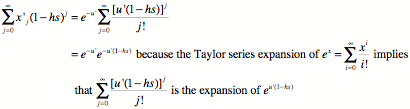
So this is the frequency of individuals with i
mutations after reproduction
and its distribution is:
![]()
The frequency of an individual
with i deleterious mutations after selection
is proportional to its frequency before selection times its
fitness. The fitness is just the
ratio of the number of xi survivors, which we get by multiplying
the frequency before selection by (1–hs)i and dividing by the
total frequency of all survivors,
which is the sum over all frequency classes of deleterious mutations:
The numerator is as follows,
plugging in the formula for the Poisson:
![]()
While
the denominator is this, pulling out a common e-u’ factor:
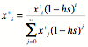
So, putting the numerator and
denominator back together we have that the frequency of the xi after
selection is as follows:
![]()
Which is simply another Poisson
distribution, with a new mean, u’(1–hs).
Substituting back for u’=uK+u,
we have that the new mean for deleterious mutations is uKnew= (uK+u)(1–hs), which makes sense: selection has shifted the
mean by reducing it a bit. This process
will continue generation after generation until we reach steady-state,
mutation-selection balance, at which point selection is removing mutations fast
enough that it balances the mutations
trickling in. At this point, uKnew = uK , i.e., we have no further change in u. Let us call the u
at this steady-state point ![]() . So we have that:
. So we have that:
![]()
Solving
this we have:
![]()
And putting this value for the
mutation-selection steady-state back into the distribution formula for x,
we have the steady-state distribution:

This is the ‘effective
population size’ reduction formula that we need to solve Problem 11.