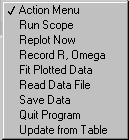
At the left is the action menu that controls what the program does. When the rotation speed has stabilized, choose Run Scope from the action menu and click the green Run button. After a second you should have a scope trace like the one below.
|
|
This web page has the LabVIEW screens from when I did the experiment.
You will obtain your own results, but I include mine here in case
you might find them useful.
Your results may be different.
At the left is the action menu that controls what the program does. When the rotation speed has stabilized, choose Run Scope from the action menu and click the green Run button. After a second you should have a scope trace like the one below. |
Here is the LabVIEW program showing a typical result of a "Run Scope" scan. This was my slowest rotational speed.
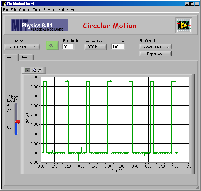
The "Record R, Omega" action on the main pull-down menus causes the program to count pulses in the graph and compute the angular velocity for the motor shaft rotation.
When you choose "Record R, Omega", the window for the scope scan on the graph will open.
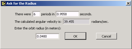
The computer has counted the number of pulses and calculated omega. (It might be a good idea to check and see if it has counted correctly.) It asks for the value of r that you have measured. When you click "OK", ω and r will be entered as x and y values in a table in the compter's memory.
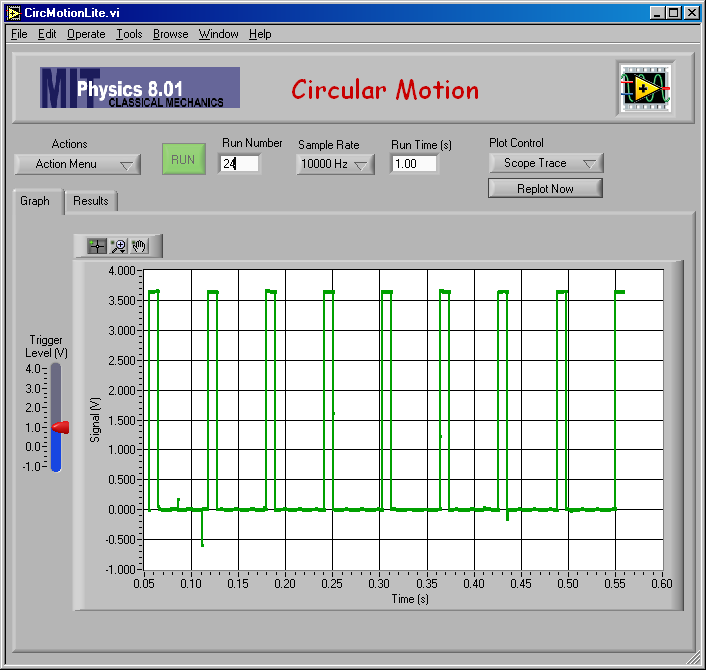
Here is my fastest rotation speed.
Make "Scope Trace" measurements to determine r and omega for four or five values of r <= 10 cm, and enter them into the table using "Record R, Omega" from the Action menu.
Then choose "R vs Omega" from the Plot Control menu and click "Replot Now" to get a graph showing your r and omega data (the green dots). Here is my plot.
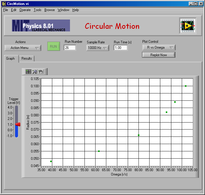
The data that are plotted on the graph can be seen in a table if you click the Results tab.
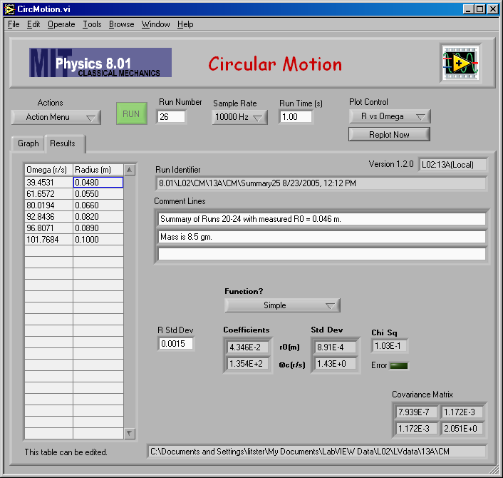
The data in the table can be edited, so that if you made any typing mistakes, when entering r for example, you can correct them. You can type over wrong values or delect and delete bad data. If you have edited the data in the table, you should replace the data in the computer's memory with those in the table by choosing "Update from Table" from the action pull-down menu. Then you should also update the graph by clicking "Replot Now".
If you change your mind and don't want to keep the changes you have made in table (or accidentally erased the table!) you can restore the table from the data in the memory by clicking "Replot Now" as long as you have not yet chosen "Update from Table" from the menu.
The r vs. ω data can be fit by the program to the function
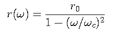
The fit is done with two adjustable parameters, r0 and ωC. Make sure the Function? pull-down menu in the middle of the Results tab says "Simple" and choose "Fit Plotted Date" from the action menu. The parameters r0 and ωC that give the best fit of the above equation to the data will be shown below the Function? pull-down menu in the table labeled Coefficients.
If you click the Graph tab, you will see that the fit equation has been plotted on the graph (in purple) along with the data points.
My result is shown on the graph below.

The equation above that was fitted to the data comes from a model that ignores the force of gravity. At small values of ω the weight will hang down slightly and follow a conical rather than a flat circular path. A model can be made to describe the motion when the force of gravity on the rotating mass is included.
The computer can fit that model to the data. It has the same two adjustable parameters r0 and ωC and if you choose Include Gravity under the Function? menu and repeat the fit, you can see how much the parameters change.
If you'd like to see a copy of my report (pdf), click this link.
J. D. Litster, October 2, 2006.