Visualizing Vector Fields
Table of Contents, Get code for this tutorial
Note: You can execute the code from this tutorial by highlighting them, right-clicking, and selecting "Evaluate Selection" (or hit F9).
This is based on a video tutorial on Doug's Video Tutorial blog.
In this section, you'll learn how to visualize vector fields. Vector fields contain vector information for every point in space. For example, air flow data inside a wind tunnel is a vector field.
Contents
Velocity Plot (Quiver Plot)
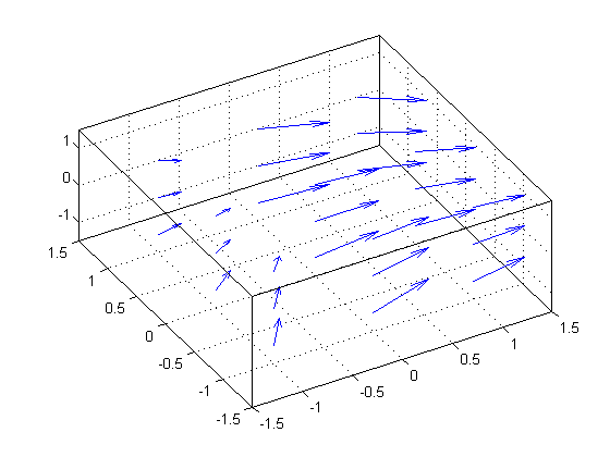
In order to visualize vector fields, you can use the quiver3 function. (For 2D, use quiver)
[x, y, z] = meshgrid([-1 0 1]);
u = x + cos(4*x) + 3;         % x-component of vector field
v = sin(4*x) - sin(2*y);      % y-component of vector field
w = -z;                       % z-component of vector field

quiver3(x, y, z, u, v, w);
axis([-1.5 1.5 -1.5 1.5 -1.5 1.5]);
view(-30, 60);
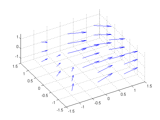
quiver3 (and quiver) places a vector at each grid point. For this reason, the visualization may not be very useful if you want a higher resolution:
[x, y, z] = meshgrid(-1.5:0.1:1.5);
u = x + cos(4*x) + 3;         % x-component of vector field
v = sin(4*x) - sin(2*y);      % y-component of vector field
w = -z;                       % z-component of vector field

% Using an invisible figure because this will choke most video cards
f = figure('Visible', 'off');
quiver3(x, y, z, u, v, w);
axis([-1.5 1.5 -1.5 1.5 -1.5 1.5]);
view(-30, 60);
print -dpng -r200 largeQuiver    % save as PNG file
close(f);
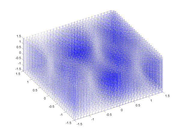
As you can see, there are too many arrows to make this a meaningful plot.
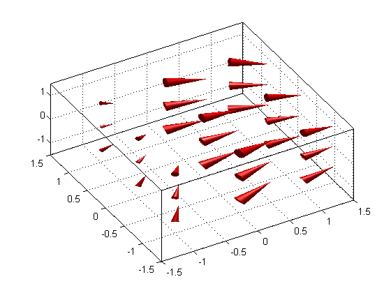
Velocity Plot (Cone Plot)
In such situations, there's a different function called coneplot that you can use. coneplot allows you to specify locations of the vectors (in the form of cones). This way, you can work with a high-resolution data without sacrificing graphics.
clf;
[x, y, z] = meshgrid(-1.5:0.1:1.5);
u = x + cos(4*x) + 3;         % x-component of vector field
v = sin(4*x) - sin(2*y);      % y-component of vector field
w = -z;                       % z-component of vector field

[cx, cy, cz] = meshgrid([-1 0 1]);
h = coneplot(x, y, z, u, v, w, cx, cy, cz, 5);
set(h, 'FaceColor', 'r', 'EdgeColor', 'none');
camlight; lighting gouraud;

grid on; box on;
axis([-1.5 1.5 -1.5 1.5 -1.5 1.5]);
view(-30, 60);
In fact, coneplot has an option to display arrows instead of cones:
delete(h)
coneplot(x, y, z, u, v, w, cx, cy, cz, 'quiver');
Streamlines
streamline gives you information about a particular particle in space and describes how it moves through the vector field.
Single Streamline
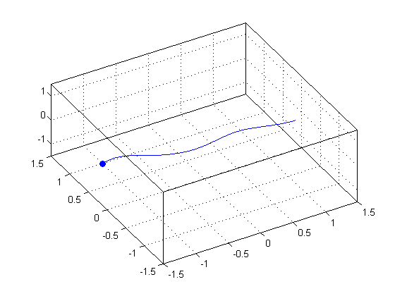
The following shows a single streamline starting at point (-1, 1, -1.5)
clf;
[x, y, z] = meshgrid(-1.5:0.1:1.5);
u = x + cos(4*x) + 3;         % x-component of vector field
v = sin(4*x) - sin(2*y);      % y-component of vector field
w = -z;                       % z-component of vector field

streamline(x, y, z, u, v, w, -1, 1, -1.5)
hold on;
plot3(-1, 1, -1.5, 'bo', 'MarkerFaceColor', 'b')

grid on; box on;
axis([-1.5 1.5 -1.5 1.5 -1.5 1.5]);
view(-30, 60);
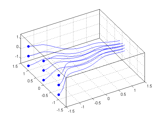
Multiple Streamlines
clf;
[sx,sy,sz] = meshgrid(-1.5, -1:1, -1:1);
hhh = streamline(x, y, z, u, v, w, sx, sy, sz);
hold on;
plot3(sx(:), sy(:), sz(:), 'bo', 'MarkerFaceColor', 'b')

grid on; box on;
axis([-1.5 1.5 -1.5 1.5 -1.5 1.5]);
view(-30, 60);
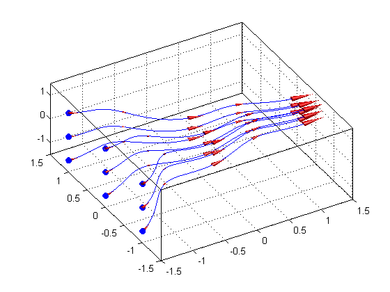
You can add velocity cones on top of the streamlines to indicate the velocity along the lines.
% Get X/Y/Z data for the stream lines
xx = get(hhh, 'XData');
yy = get(hhh, 'YData');
zz = get(hhh, 'ZData');

% Place 5 velocity cones per stream line
fcn = @(c) c(round(linspace(1, length(c), 5))); % index into 5 equally spaced points
xx = cellfun(fcn, xx, 'uniformoutput', false);
yy = cellfun(fcn, yy, 'uniformoutput', false);
zz = cellfun(fcn, zz, 'uniformoutput', false);

hhh2 = coneplot(x, y, z, u, v, w, [xx{:}], [yy{:}], [zz{:}], 2);
set(hhh2, 'FaceColor', 'r', 'EdgeColor', 'none');
camlight; lighting gouraud;
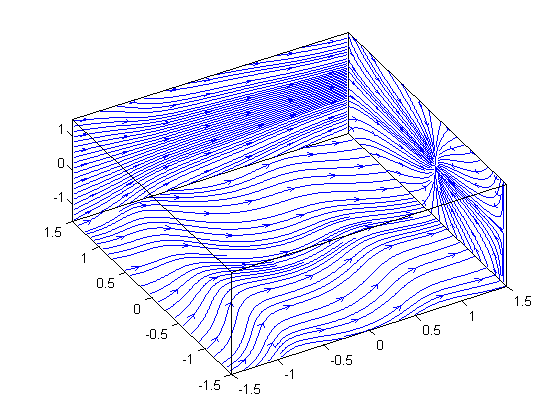
Streamslice
streamslice works very similarly to slice and allows you to cut a plane through the space and project the vector field onto it.
clf;
[x, y, z] = meshgrid(-1.5:0.1:1.5);
u = x + cos(4*x) + 3;         % x-component of vector field
v = sin(4*x) - sin(2*y);      % y-component of vector field
w = -z;                       % z-component of vector field

streamslice(x, y, z, u, v, w, 1.5, 1.5, -1.5);
box on;
axis([-1.5 1.5 -1.5 1.5 -1.5 1.5]);
view(-30, 60);
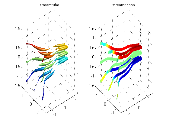
Stream Tube and Stream Ribbon
A couple of other vector field visualization tools to keep in mind are streamtube and streamribbon. streamtube allows you to visualize the normalized divergence of the vector field, while streamribbon is proportional to the curl of the vector field. See the documentation for more information.
clf;
[x, y, z] = meshgrid(-1.5:0.1:1.5);
u = x + cos(4*x) + 3;         % x-component of vector field
v = sin(4*x) - sin(2*y);      % y-component of vector field
w = -z;                       % z-component of vector field
[sx, sy, sz] = meshgrid(-1.5, -1:1, -1:1);  % stream starting point

% streamtube
subplot(121);
streamtube(x, y, z, u, v, w, sx, sy, sz);
shading interp
axis([-1.5 1.5 -1.5 1.5 -1.5 1.5]);
camlight; lighting gouraud
grid on;
title('streamtube');

% streamribbon
subplot(122);
streamribbon(x, y, z, u, v, w, sx, sy, sz);
shading interp
axis([-1.5 1.5 -1.5 1.5 -1.5 1.5]);
camlight headlight; camlight right; lighting gouraud
grid on;
title('streamribbon');