Introduction

There are also a few factors that we considered that related more to the subject’s internal state than the reward received from the game. 

Time
We informally called this the “boredom factor.”  If the subject is getting tired of pressing buttons or feels like a long time has elapsed, they may start to press buttons faster and to think less about optimizing their reward.  Because of the structure of the reward curves, this may inadvertently help them optimize their reward if they press a single button repeatedly.

Motivation
In the initial phase of our study, we found that subjects were less engaged in the task and seemed to just want to get it over with.  After re-working the instructions and changing the interface to allow for more instantaneous reward, we saw what we thought to be an increase in subject motivation.  They seemed to be more excited about the experiment and to think more about each choice.

Risk aversion
We considered this to be a personality trait that is difficult to assess or control for. A person who is more risk averse would be less likely to explore or deviate from a button-pressing strategy that seemed to give consistent rewards.

Approach

Our approach concerns modeling user behavior based on reward history. At each time, t, there is a history vector, xt, which is an n+2 dimensional vector consisting of the current trial number, the total accumulated reward, and the past n rewards received.

Mathematically, this vector looks like

xt = [rt, rt-1, ..., rt-n+1, t, Rt],    where Rt = r1+r2+...+rt

Initially, we considered several simple ways of using the history vectory to analyze switching. Some of these are discussed below

Immediate reward delta
If we base our switching decision st solely on whether or not our reward increased as a result of our last action, the relevant metric can be expressed as

f(xt) = w'xt,    w= (1, -1, 0, ..., 0, 0, 0)

A positive f(xt) indicates that the last action led to a reward increase. A negative f(xt) indicates that the last action led to a reward decrease. We might hypothesize that the subject is more likely to switch when f(xt) is negative, and less likely to switch when f(xt)

Average reward delta
A simple variant of the previous approach is to consider the average change in reward over the last $n$ actions. In this case, the switching metric can be expressed as

f(xt) = w'xt,    w= 1/n (1, 0, 0, ..., -1, 0, 0)

Accumulated reward
Another factor to consider is the overall reward accumulated so far.

f(xt) = w'xt,    w= (0, 0, 0, ..., 0, 0, 1)

Discriminant Analysis

Each of the functions described in the previous section was a linear combination of the components of xt and used a specific set of weights in a parameter vector w. This parameter vector specifies the relevance of each component in the final score. Instead of relying on an arbitrary weight assignment, we would like to find an optimal w for each subject by using statistics obtained from their past actions. From a pattern classification perspective, we can accomplish this by using linear discriminant analysis (LDA) on the history vectors.

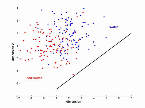
Figure 1 - Example set of vectors from two classes. Black line
indicates optimal projection vector

First we designate a group of history vectors as the training set. Separate the history vectors into two classes, "switches" (C1) and "non-switches" (C0). The optimal w will project the vectors in C1 and C0 into scalars whose class means are well separated and whose class variances are small. Intuitively, this means we want the projected scalars from one class to be clustered together and far away from the other class. Mathematically, we are trying to maximize

distance between projected means = |w'm1-w'm0|

and minimize

overall within class variance, Sw= w'Var(C1)w + w'Var(C0)w

The solution to this optimization [1] is

w* = inv(Sw)(m1-m0)

Once the weight vector is determined, we project all history vectors into scalars and use a normal distribution to model each of their condition probabilities

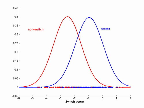
Figure 2 - Distribution of points after being projected into single
dimension.

For an incoming history vector xt, we can calculate the class conditional probabilities based on the distributions that were estimated during training. Thus

p(xt|Switch) = N(w*'xt; w*'m1, w*'Var(C1)w*)

p(xt|Non-Switch) = N(w*'xt; w*'m0, w*'Var(C0)w*)

If we are simply performing classification, then we use the decision rule

If we are using the model to play the game, and we want to incorporate some degree of randomness into the choice, then we use Bayes' rule to compute the probability of switching.

We then allow the model to switch or not according to this probability.

Evaluation Paradigm

We decided to evaluate our model by using a split classification scenario, in which the w vector was trained on the first half of a trial, then tested/compared to the last half of the trial. The purpose of this evaluation paradigm was to remove variabilities across subjects and across reward functions for the different methods. In particular, we looked at two ways of comparing model behavior with subject behavior. In each of our evaluations we used a 7 dimension history vector which had 5 past rewards, the current value of t, and the accumulated reward.

Prediction
The first testing method involved using the model to continue playing the game for the last half of the trial. Under this scenario, the reward history generated by the model's actions may diverge from the reward history actually experienced by the subject, so it is important to distinguish this type of test from the classification task described next.

We evaluated the performance of our model on this task by measuring how far the model ended up from where the subject actually ended up. Since the action trajectory of the model is, by nature, stochastic, we allow the model to play the game multiple times and average the final deviation errors.

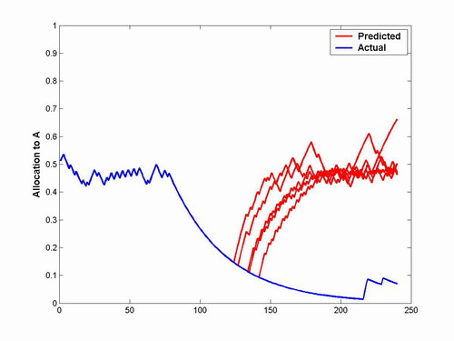
Figure 3 - Example allocation trajectories predicted by model playing the
game compared to actual allocation trajectory followed by user. Deviation
error is calculated by the difference in allocations on the final trial.

Classification
The second testing method involved simply classifying all subsequent user actions in the last half of the trial as "switch" or "non-switch" based on the reward history generated by the user himself.

We evaluated the performance of our model on this task by simply calculating the error rate which is given by the number of misclassified history vectors over the total number of history vectors classified.

Results

For the prediction task, we let the model "continue the play" five times for each subject and method and computed the average difference between the final allocation points of the subject and the model.

For the classification task, we obtained the following switch classification error rates:

Matlab Code

REQUIRED TOOLBOX FOR ANALYSIS
For the purposes of this project, we used the Discriminant Analysis Toolbox for Matlab authored by Michael Kiefte from the University of Alberta. This toolbox is available from the Matlab Central File Exchange at the following location.

The following files were used to perform analysis and training. Each function has appropriate documentation that can be viewed by typing "help <function_name>".

References