Alternation in the repeated Battle of the Sexes

Aaron Andalman & Charles Kemp
9.29, Spring 2004
MIT

Abstract:

Traditional game-theoretic models consider only stage-game strategies. Alternation in the repeated battle of the sexes is a robust empirical finding that defies explanation by these simple strategies. We consider a natural extension of stage-game strategies -- Hidden Markov models with two states -- and develop a belief-learner that alternates in self-play and when playing against humans.

Introduction

Consider two employees who commute to the same workplace. Both prefer to travel in the same car because they save gas money and enjoy the company, but both enjoy the journey most when the other person drives. Each morning when the employees assess their transport options they play a version of the ``Battle of the Sexes'' (see Table 1).

This game pits cooperation against the desire to achieve the maximum reward on each move. Both players maximize their payoff by coordinating their play and choosing the same strategy. Each player, however, prefers a different strategy. This situation is common in everyday social settings, and in many cases the game is played repeatedly by the same group of players.

Table 1: Battle of the Sexes payoff matrix.

	My Car	Your Car
My Car	1,2	0,0
Your Car	0,0	2,1

The behavioral patterns that humans exhibit in repeated play were recently studied by McKelvey and Palfrey (2). They show that subjects playing repeated Battle of the Sexes often fall into a stable pattern of alternation between the two pure-strategy Nash equilibria (see Figure 1). Alternation is a simple strategy that seems intuitive in real-life situations such as our carpool scenario. Standard learning models, however, are unable to account for this behavior.

Figure: Repeated ``Battle of the Sexes'' often results in alternation. Each point shows the average payoff for a pair of players after 50 rounds. The payoff matrix was $$\begin{bmatrix}18,6 & 3,3 \\ 3,3 & 6,18 \end{bmatrix}$$, and the cluster at $[12,12]$ reflects alternating play. The purple dots are the Nash Equilibria. The triangle encloses the regions of reward space which can be achieved in principle. (Reproduced from (2).)

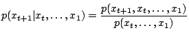
Most learning models consider stage-game strategies. Each player maintains a probability distribution $P$ over all his possible moves, and once equilibrium has been reached a player's move at time $t+1$ is conditionally independent of his previous move given $P$. A natural way to allow the possibility of alternation is to give a stage-game player two or more internal states. Now the player maintains $n$ probability distributions, one per state, and we must specify how the player moves between states.

Many of the traditional questions that have been asked about stage-game learners carry over to learners with internal states. One issue that has been extensively explored with simple learners is the difference between reinforcement learning and belief learning. A reinforcement learner is concerned only with its own history of moves and payoffs, and tends to choose strategies that have worked well in the past. A belief learner models its opponent directly, and chooses its own move based on a prediction about the opponent's next move. Hanaki and colleagues have recently described a reinforcement learning model that considers learners with internal states (1). In this paper we develop a belief learner that models its opponent as a player with internal states. Our primary goal is to develop a learner that can alternate when playing itself and when pitted against a human.

Model

We developed several belief-learners that model their opponents using hidden Markov models (HMMs) with two states. A two-state HMM has five parameters:

• $p_1$, the probability that the model starts out in state 1

• $q_{11}$ and $q_{22}$, where $q_{ii}$ is the probability that a learner in state $i$ at time $t$ remains in state $i$ at time $t+1$

• $o_{11}$ and $o_{22}$, where $o_{ii}$ is the probability that a learner in state $i$ chooses move $i$

A one-state HMM plays a stage-game strategy -- it chooses each move with a flip of a biased coin. Most previous work on belief learning has considered models of this sort. In particular, fictitious play amounts to modeling one's opponent with a one-state HMM. Working with two-state HMMs maintains continuity with this previous work but expands the set of possible strategies.

Each of our learners is a combination of two components: a strategy for predicting the opponent's next move and a decision rule that chooses a move based on this prediction. We introduce two predictive strategies and two decision rules.

Predictive Strategies

We impose a memory restriction to allow the learners to respond quickly to nonstationary opponents. Each predictive strategy takes only the previous $n$ moves into account. Following Miller's research on human short-term memory, we set $n=7$.

Bayesian integration

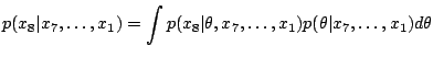
A full Bayesian learner begins with some prior distribution over the space of HMMs and predicts its opponent's next move by integrating over this space. Suppose that the opponent chooses move $x_i$ at time $i$. Then the distribution for $x_{t+1}$ is

$$p(x_{t+1}\vert x_t, \ldots, x_1) = \frac{p(x_{t+1}, x_t, \ldots, x_1)} {p(x_t, \ldots, x_1)}$$ (1)

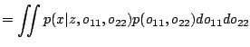
Suppose $x=\{x_1, \ldots, x_t\}$ and $z=\{z_1, \ldots, z_t\}$, where $z_i$ is the hidden state of the opponent at $i$. Then $p(x)$ can be computed by summing over all possible hidden state sequences $z$:

$$p(x) = \sum_z p(x\vert z) p(z)$$ (2)

The memory restriction limits the length of the sequences $z$ that must be considered and makes it possible to compute this sum. We show how to compute $p(x\vert z)$: $p(z)$ can be computed similarly.

Given $x$ and $z$, suppose that $m_{ij}$ is the number of times the opponent played move $j$ when in state $i$.

$$p(x_8\vert x_7, \ldots, x_1) = \int p(x_8\vert\theta, x_7, \ldots, x_1)p(\theta\vert x_7, \ldots, x_1) d\theta$$ (3)

$$p(x\vert z) = \iint p(x\vert z, o_{11}, o_{22}) p(o_{11}, o_{22})do_{11} do_{22}$$

$$= \iint o_{11}^{m_{11}}(1-o_{11})^{m_{12}} (1-o_{22})^{m_{21}}o_{22}^{m_{22}} p(o_{11}, o_{22}) do_{11} do_{22}$$

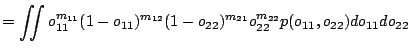If we use independent beta priors with parameters $\alpha$ and $\beta$ for $o_{11}$ and $o_{22}$ it is straightforward to show that:

$$p(x\vert z) = \left( \frac{\Gamma(\alpha+\beta)}{\Gamma(\alpha)\Gamma(\beta)}... ...\Gamma(m_{21}+\alpha)\Gamma(m_{22}+\beta)}{\Gamma(m_{21}+m_{22} +\alpha+\beta)}$$

For each of the five parameters we use a uniform prior distribution ( $\alpha=\beta=1$).

Point estimates: EM

Instead of integrating over the space of HMMs, the opponent's move can be predicted using a single HMM that describes his previous moves well. A suitable HMM can be found using the EM algorithm. The algorithm starts off at a random setting of the HMM parameters, and iteratively improves them until it reaches convergence. It may not find the best HMM overall, but is guaranteed to converge to a local maximum of the posterior density. Unlike Bayesian integration, the EM algorithm is relatively efficient and can be used even when memory capacity is increased well beyond seven units.

In psychological terms, an EM player is a player who jumps to one plausible explanation for his opponent's behavior and fails to consider other potential explanations. We ran EM with 5 random restarts. If enough random restarts are used, EM will find the best HMM with high probability, but with only 5 restarts EM may settle on a HMM that is good, but not ideal.

Decision Rules

Given a prediction about the opponent's next move, a maximizing rule chooses the response that maximizes expected income on the next move. A matching decision rule chooses between the moves in proportion to their expected payoffs on the next move. The maximizing rule is deterministic (in the absence of ties), but the matching rule is stochastic.

Results

The combination of two predictive strategies and two decision rules produces four players. Each player has the capacity to alternate, and will use this capacity whenever it decides with high probability that its opponent is alternating. Whether alternation emerges in self-play is another matter entirely.

Self-Play

Alternation in self-play is a demanding test of a learning algorithm. Considerations of symmetry show that alternation can never emerge between identical deterministic players. The symmetry problem is a challenge for all approaches, but self-play also introduces problems for belief learners in particular. When playing itself, a belief-learner can never form a perfectly accurate model of its opponent. Attempting to build such a model leads to an infinite regress: player A's move depends on B's move which depends in turn on A's move, and so on.

Alternation in self-play might therefore seem like a quixotic goal. It never occurs on truly principled grounds, and will only be seen if randomness pushes a pair of identical players in the right direction. Even so, different strategies for including randomness can be more or less psychologically plausible. A player that chooses its first five moves at random but is otherwise deterministic might sometimes achieve alternation, but seems less humanlike than a player that uses a stochastic decision rule throughout. Incorporating randomness in a psychologically plausible manner is a worthy challenge.

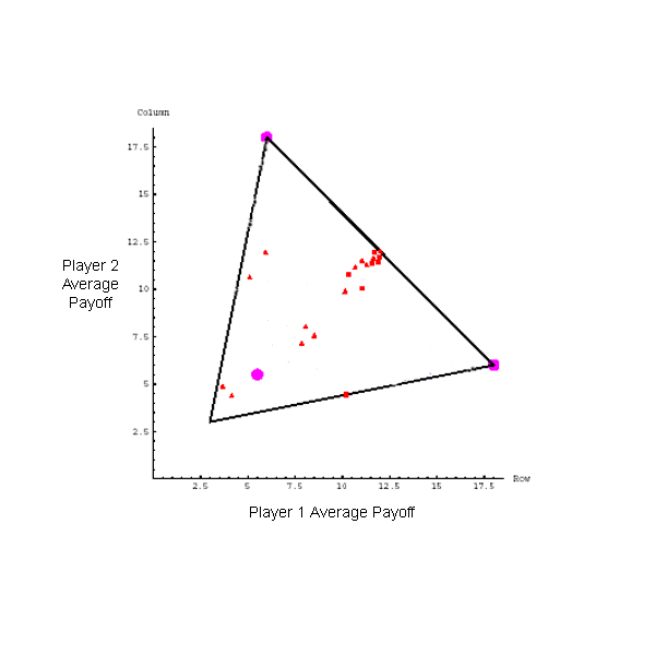
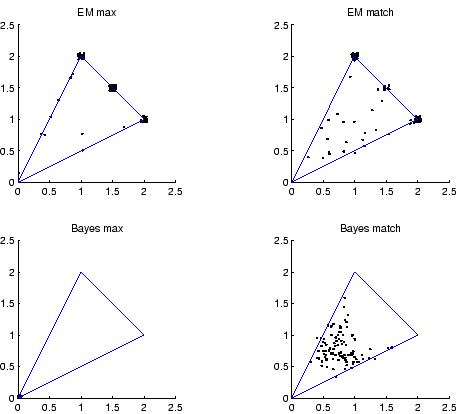
Figure 2 summarizes the patterns of play when each of our models is played against itself. Each model played 100 50-move matches against itself, and each point plotted shows average rewards over the last 20 moves of a 50-move match. Points near $(1.5, 1.5)$ represent matches where the players succeeded in alternating.

The top left plot shows that the maximizing EM player often alternates when pitted against itself. This player uses a deterministic decision rule, so the symmetry between the players can only be broken if EM sometimes falls short of the true MAP parameter estimates. Some sequences of moves are assigned approximately the same probability by several different HMMs, and the EM algorithm may settle on any of these.

Analyzing individual matches shows that alternation occurs most often when player 1 has played $[2,1,2,2]$ and player 2 has played $[1,2,1,1]$. Imagine this situation and put yourself in the position of player 2. Table 2 shows two HMMs that model your opponent's moves. If you choose the second HMM, you should play 1 on the next move since you are using the maximizing decision rule. But if you choose the first HMM, you should play 2, since $2*P($opponent plays 1$) < P($opponent plays 2$)$. Note that the log likelihoods of these two HMMs are close to identical.

Table 2: Two possible inferences about the move history $[2,1,2,2]$. $p$, $O$ and $T$ are the prior state distribution, observation matrix and transition matrix respectively. Given these parameters, $LL$ is the log likelihood of the move history and the final column shows predictions about the opponent's next move.

	$p$	$O$	$T$	$LL$	next move
Estimate 1	$\begin{bmatrix}0 \\ 1 \end{bmatrix}$	$\begin{bmatrix}0.74 & 0.26 \\ 0 & 1 \end{bmatrix}$	$\begin{bmatrix}0 & 1 \\ 0.67 & 0.33 \end{bmatrix}$	-1.3864	$\begin{bmatrix}0.32 \\ 0.68 \end{bmatrix}$
Estimate 2	$\begin{bmatrix}0 \\ 1 \end{bmatrix}$	$\begin{bmatrix}1 & 0 \\ 0 & 1 \end{bmatrix}$	$\begin{bmatrix}0 & 1 \\ 0.5 & 0.5 \end{bmatrix}$	-1.3863	$\begin{bmatrix}0.5 \\ 0.5 \end{bmatrix}$

The remaining three plots in Figure 2 show that the matching EM player sometimes alternates, but neither of the integrating players succeeds in alternating. The maximizing integrating player does particularly poorly when played against itself. Since this player is deterministic, a symmetry argument shows that it can never achieve any reward.

A comparison between the matching EM player and the matching integrating player is particularly interesting. The crucial difference between the two is that the EM player considers only one explanation for the opponent's behavior, but the integrating player considers many. Jumping to a premature conclusion may not be theoretically optimal, but it does seem psychologically plausible. Without this property, the integrating Bayesian learner can only achieve alternation in self play if we increase the prior probability assigned to HMMs that alternate.

Figure 2: Average rewards when each player plays itself. Each point shows average rewards over the last 20 moves of a 50 move match. Random jitter has been added to each point so that the size of each cluster is visible.

Human opponents

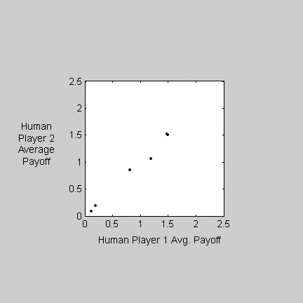
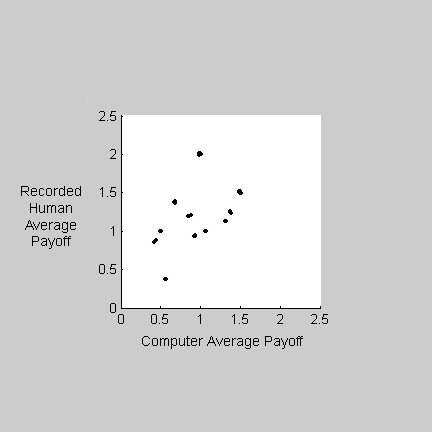
Both the EM players will alternate against a human player who is determined to alternate, and so will the integrating players if we increase the memory size beyond seven. We collected data from 16 subjects (8 pairs) playing each other in Battle of the Sexes (Figure 3a) and played the maximizing EM model against each subject's recorded moves (Figure 3b). The cluster of points near [1.5,1.5] in Figure 3b shows that our EM model alternates against recorded human data. However, the subjects may have played differently when faced with our model's choices.

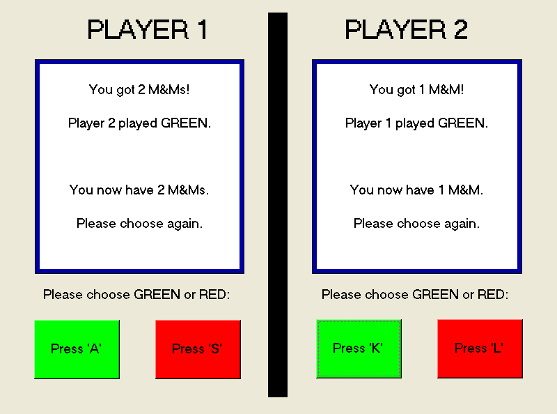
To address this possibility, we asked three experimental subjects to play the maximizing EM player directly. One out of the three fell into a stable pattern of alternation. Even though the sample size is tiny, this result shows that the maximizing EM player can indeed alternate when played in real time against a human.

Our model is more willing than humans to be exploited by its opponent. This problem can be seen in figures 2 and 3(b), which show clusters of points at the opponent's preferred pure strategy Nash equilibrium. Figures 1 and 3(a) suggest that human players rarely give in to such exploitation. Humans rarely allow each other to get away with unfair rewards.

Figure: Average rewards for (a) humans versus humans and (b) maximizing EM model versus recorded human data. Payoffs are averaged across the final 15 rounds of play.

Discussion

The maximizing EM player is a belief learner that alternates when playing itself and humans in the repeated Battle of the Sexes. This player should also perform sensibly when asked to deal with other payoff matrices. Regardless of the game, the maximizing decision rule means that it will always choose the optimal response when playing a pure-strategy opponent. Provided that we endow it with a large enough memory, it will converge to optimal play when pitted against any opponent playing a stage-game strategy (mixed or pure).

Our belief-learning approach overcomes some of the limitations of Hanaki's model, which performs reinforcement learning over the set of all two-state deterministic finite automata. Our model alternates right out of the box, but Hanaki's model requires a long run `pre-experimental' phase before it is ready to alternate. Hanaki's algorithm enumerates all deterministic two-state automata, and therefore does not scale easily to automata with more than two states. Our probabilistic approach can readily handle automata with many internal states.

It is not clear that the maximizing EM player alternates for the right reasons. People may alternate because alternation is the best sustainable strategy. To return to our carpool scenario, I might prefer it if you drove me to work every day, but our friendship is unlikely to survive if I try to force you into this equilibrium. Our model, however, has no notion of a sustainable strategy - it just tries to achieve the best possible reward on the next move. A more sophisticated belief learner might address this weakness by considering the effect of his own moves on his opponent's play. This approach, however, leads directly to the infinite regress mentioned previously. Adding some notion of fairness to the model might also address this shortcoming, but fairness is difficult to formalize in a principled way.

Even though alternation in the Battle of the Sexes is just one of many game theoretic phenomena, we believe that it raises an important general point. Alternation is a strategy that is intuitive and simple, but even so it is beyond the scope of most traditional learning models. Attempting to characterize and work with the class of strategies that people actually consider is an important project for behavioral game theory.

Experimental Methods

We ran a total of 19 subjects in repeated Battle of the Sexes experiments. Eight games of human versus human play were recorded, and three games of human versus our model. All data was collected using a Matlab graphical user interface (see Figure 4). Prior to each game, instructions were displayed in text and read aloud. Subjects were asked not to communicate with their opponents. The payoff matrix in Table 1 was used in all games. Each game consisted of 30 rounds. During each round subjects selected a strategy, either red or green, by pressing a key. The keyboard was hidden from view to prevent subject seeing each other's moves. After each round the two players' selected strategies, current payoffs, and cumulative payoffs were displayed. At the end of the game, each subjects rewards were provided in the form of M&M candies.

Figure: Matlab program for data collection.

Acknowledgments

Tom Griffiths showed us that full Bayesian integration is possible for a memory-limited player. All of our models were developed using Kevin Murphy's HMM toolbox.

Bibliography

1

N. Hanaki, R. Sethi, I. Erev, and A. Peterhansl.
Learning strategies.
Journal of Economic Behavior and Organization, 2004.
In press.

2

R. D. McKelvey and T. R. Palfrey.
Playing in the dark: Information, learning and coordination in repeated games.
Technical report, California Institute of Technology, 2001.