Reinforcement learning in a Simple Game
Seungeun Oh
Yonatan Loewenstein
Abstract
Abstract |
Introduction |
Methods |
Results |
Discussion
The purpose of this project is to see to what extent and how a model based on the reinforcement learning theory fits real human behavior.
We had 20 pairs of people play penny-matching against each other.
Resorting to the reinforcement learning theory, we assume that each player holds a policy, a method of choosing actions, and modify their policy as they learn from their past experience. Observed behavior of players show that the policy is stochastic but has deterministic, win-stay-lose-switch bias.
To discover the learning rule, we look for the correlation of action and history in terms of eligibility trace. But consistent trend was found only when we relate action to the immediate past.
The policy indexed by probability showed large oscillation in time.
If this oscillation is chaotic or means something else is left to future work.
Introduction
Abstract |
Introduction |
Methods |
Results |
Discussion
Matching law has been observed in animal behavior, and is not always optimal.
This suboptimality can be understood by reinforcement learning theory,
it isinterpreted as deviation from maximum due to finite length of memory.
Policies are parameterized by a probability p (0<=p<=1) and
learning parameter is selected.
Continuous spectrum of policy from matching to maximizing can be reached by varying p.
Here we analyze data of human behavior in a simple game quantitatively
to verify the scope of the reinforcement learning theory.
Methods
Abstract |
Introduction |
Methods |
Results |
Discussion
Game description
Two people sit in front of a computer and choose either side of a coin by pressing keyboard. In deterministic pennymatching one wins if two people chose the same side while the other wins if they chose different sides from each other. Here we used pennymatching payoff matrix with perturbative randomness. The payoff matrix elements stand for players' probability of winning.
|
Payoff
Matrix
|
Player2 matcher
|
|
0
|
1
|
player1
non-matcher
|
0
|
(1/4,3/4)
|
(3/4,1/4)
|
|
1
|
(3/4,1/4)
|
(1/4,3/4)
|
Game code : C. Curses library required.
Analysis methods
We will use a boxcar filter of specified length in calculating probability p and p from sequence of choices.
p will stand for the probability of choosing action 1 while p=1-p will stand for the probability of choosing action 0.
The equilibrium would be mixed strategy of 0.5 probability for both action.
This is Nash equilibrium and matching at the same time.
- Phenomenological approach
-
- Comparison with random data
- Seeking tendencies and patterns
-
- Model based approach
-
- Interpretation as reinforcement learning
-
-
Results
Abstract |
Introduction |
Methods |
Results |
Discussion
data
We collected 20 sets and each game consists of 500 turns. A game takes about 10~15 minutes.
Set 4 is bad to the end and set 9 is exceptional because player 2 knew the payoff matrix in advance and cheated by looking at the other player's hand.
data files : choice history,
reward history
Non-equilibrium behavior
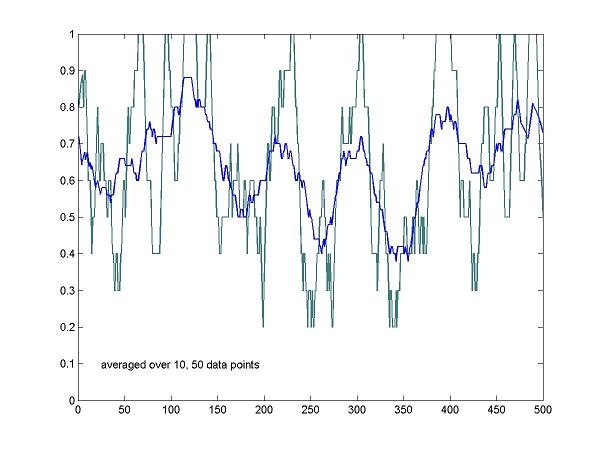
The policy or probability p as defined above, depends on the length of the filter.
Figure shows fluctuation of p of a player by filter length of 10 and 50.
There's large fluctuation of the probability regardless of the choice of the filter length. The probabilities do not converge to the Nash equilibrium.
Similar plots of other game sets calculated by various filter lengths; 30, 60, 90, 180.
set1,
set2,
set3,
set4,
set5,
set6,
set7,
set8,
set9,
set10
matlab code : This function filters binomial choice history with normalized boxcar filter of specified length.
Deviation from Nash equilibrium
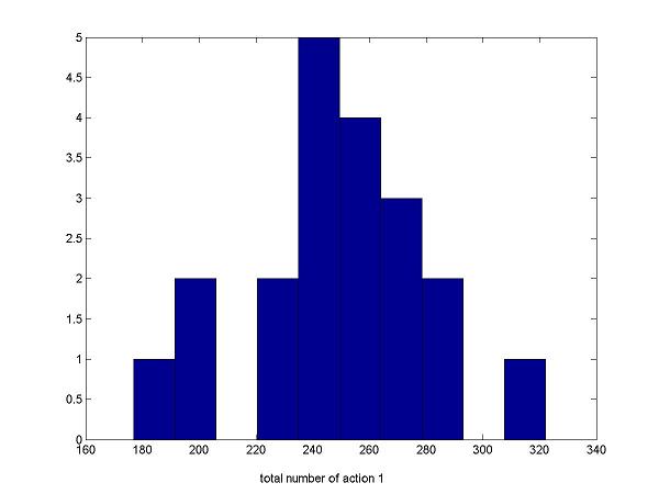
If people were approaching the Nash equilibrium p=0.5, they would have chosen both choices by almost the same frequency. In the ideal case, the mean of the number of action 1 is 250 out of 500 trials and the standard deviation is approaximately 11.
Following histogram is the number of choice 1 versus number of players. It shows that many people were biased toward either choice
beyond the standard deviation from the mean.
Randomness of actions
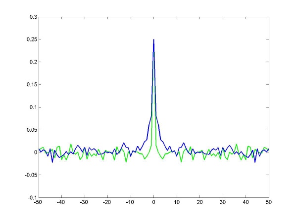
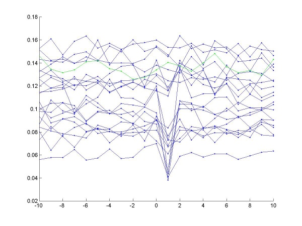
Compared to the truly random sequence(green line), human behavior have character dependent bias.
Figure is the plot of auto-correlation of choices.
Wider center peak than that of random sequence implies player's tendency to choose the same action continuously,
while negative peaks right next to the center peak mean that the player tends to alternate.
data from other games
Bias toward deterministic behavior (1: Win-stay-lose-switch policy)
Win-stay-lose-switch policy was observed in many games.
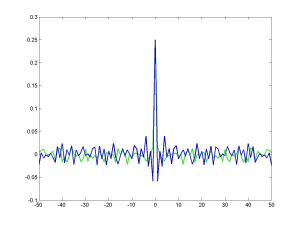
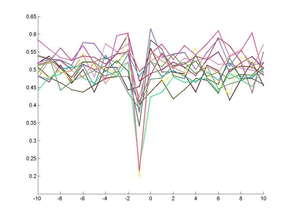
We can calculate switch-averaged income to see what income makes people change their choices.
In the following figure x-axis is time and origin is when they made a choice different from the previous one.
Y-axis is income which is around 0.5 by average.
Large negative peak just before origin is a prominent evidence supporting that many players switch their choices just after losing.
By choosing a filter of length 2, we can have the variation to reflect the change of choices. The variation is 0 if the two consecutive actions are same
while, it is 0.25 if they are different.
Then the income averaged variation indicates if people change from whatever choice they made before. In the figure, the origin is the time when they won.
Negative peaks right after origin mean that not all but some players stayed with their choice after winning.
In short win-stay-lose-switch behavior is observed. We will see in the next paragraph how dominent this deterministic policy is.
Bias toward deterministic behavior (2: Degree of the bias)
We assumed that a player choose either action probabilistically and independent of previous choice according to p.
If that hypothesis works, the number of win-stay-lose-switch sequences will be approximately same as that of win-switch-lose-stay sequences when p=0.5.
Here we calculated the percentage of win-switch-lose-stay sequences in the sections of the sequences where approximately p equals 0.5.
The length of section with p between 0.495 and 0.505 is as follows for each player's game.
172, 71, 196 , 127 , 137 , 119 , 78 , 87, 200, 161, 134, 111, 47, 109, 88, 99, 69, 94, 81, 73 out of 500 trials
And the temporal distribution of such behavior is rather uniform.(data not shown)
If plays are indeed stochastic, the percentage would be 50%.
The error bar is the width of standard deviation from 50%.
18 out of 20 players lie below 50% and about 7 players far below compared to the standard deviations.
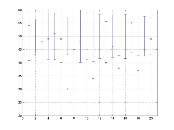
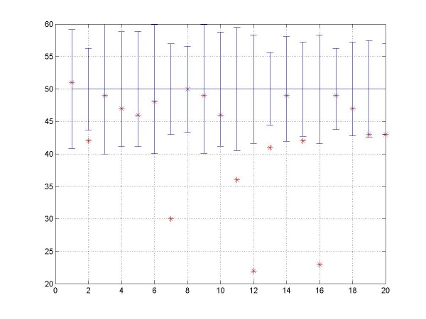
Furthermore, such tendency is persistent throughout the game.
The percentage of
win-switch-lose-stay sequences calculated over the whole sequence instead of p=0.5 portion is plotted below.
Though less clear, the overall downward shift persists.
Discussion
Abstract |
Introduction |
Methods |
Results |
Discussion
The bias toward win-stay-lose-switch policy is necessary
Our claim is that such bias is a necessity to make the policy searching algorithm work.
If we define eligibility at trial t as below,
it measures the deviation of actions from the policy, p.
et = pt at - pt at
= (1-pt) at - pt (1-at)
= at-pt
= pt (1-at) - (1-pt) at
= pt-at
Learning rule is, roughly speaking, that a deviation is reinforced if it resulted in positive income, and suppressed if resulted in negative or zero income.
This can be formulated in many ways. For example,
delta qt =
delta log(pt/pt) = ht
et
Eligibility trace et is weighted sum of eligibilities.
ht obsorbed any multiplicative constant.
Then the effect of the eligibility on the magnitude of change due to a single step of learning is smaller change in p for smaller deviation from p.
at is close to pt very often.
et = at-pt
is small most of the time.
delta qt is small.
pt changes by small amount.
The policy will be stuck at one of the edges p=0 or p=1 where actions are highly coherent with policy.
This kind of algorithm is good at converging if the learner is on the right tract but bad at rebounding the learner from a wrong track.
Theoretically, there can be many possible ways to escape the traps at p=0,1.
One can constrain p between 0.05 and 0.95 or adjust definition of q such that
change in q is amplified if p is around 0 or 1.
Another way to fix it is to strengthen 'lose-change of the policy' factor in the algorithm. Our experiment supports the latter. 'lose-change of the policy' feature is not only strengthened near p=0 and 1 but is always there for any value of p. Hence one way to incorporate this is modifying the learning rule to,
delta qt =
ht et
+ n * hti(at-at)
where the constant factor n indicates the strength of win-stay-lose-switch policy and may vary from person to person.
On the other hand, it is possible to redefine policy as a mixture of probabilistic and deterministic ways of choosing actions.
Causality between choice sequence and income sequence
As shown above the most prominent causal relation is win-stay-lose-switch.
This policy requires the information of one step past only.
Here we look for a causal relation of longer time scale.
First approach is to calculate
ht et
and delta pt from experimental data
and to examine how their covariance. Another way is to assume linear filter
between them and calculate the kernel which would be constant times weighting factors in eligibility trace. But both analysis failed to reveal any clear feature.
Long time scale oscillation
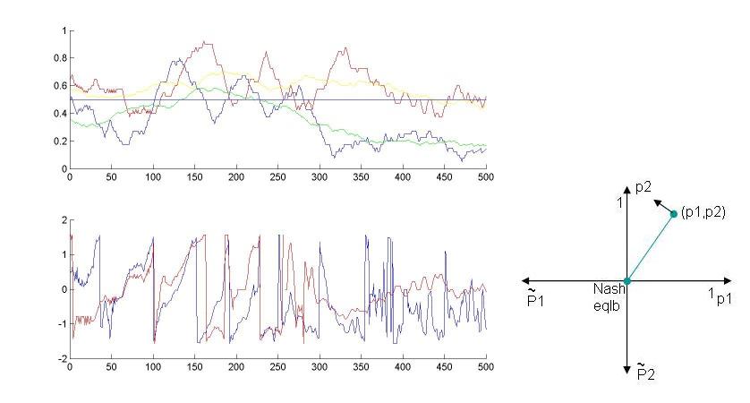
From the payoff matrix we know that the matcher will try to do like the non-matcher, while the non-matcher will try to do differently from matcher.
In the first half of the game set 7, we could observe such behavior.
Following figure is probability of non-matcher (blue) and matcher (red).
Second figure is plot of the angle in phase space (different colors for different filter lengths). We can see that the phase increase in an almost constant velocity from t=50 to t=200. But overall, this phenomena was not very general and it is possible that people couldn't learn enough to converge to the Nash equilibrium and showed such large fluctuations.
set1|
set2|
set3|
set4|
set5|
set6|
set7|
set8|
set9|
set10
Note on future works
We suggested a modification of learing algorithm or policy to explain our experimental data.
It must be interesting to investigate literature to check what specific learning algorithm or policy
can actually fit experiments.
The long term oscillation of probability was interesting but hard to understand.
If we give little more information to the players and players converge to the equilibrium strategy, then we might be able to see the oscillation transiently.
Abstract |
Introduction |
Methods |
Results |
Discussion
Game design: Group
Matlab coding and analysis: Seungeun Oh (^_^)
Thanks to Yonatan for the discussions and advice.