Electrostatics

The governing equations of electrostatics are

$$\boldsymbol{ E} = - \nabla V$$ (102)

and

$$\nabla \cdot \boldsymbol{ E} = \frac{\rho^e}{\epsilon_0},$$ (103)

where $\boldsymbol{ E}$ is the electric field, $V$ is the electric potential, $\rho^e$ is the electric charge density and $\epsilon_0$ is the permittivity of free space ( $\epsilon_0=8.8542 \times 10^{-12} ~$   C$^2/$Nm$^2$). The electric field $\boldsymbol{ E}$ is the force on a unit charge.

In metals, it is linked to the current density $\boldsymbol{ j}$ by the electric conductivity $\sigma_c$ [5]:

$$\boldsymbol{ j} = \sigma_c \boldsymbol{ E}.$$ (104)

In free space, the electric field is locally orthogonal to a conducting surface. Near the surface the size of the electric field is proportional to the surface charge density $\sigma$[21]:

$$\sigma={ E}_n \epsilon_0.$$ (105)

Substituting Equation (102) into Equation (103) yields the governing equation

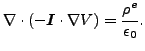$$\nabla \cdot (- \boldsymbol{ I} \cdot \nabla V) = \frac{\rho^e}{\epsilon_0}.$$ (106)

Accordingly, by comparison with the heat equation, the correspondence in Table  (13) arises. Notice that the electrostatics equation is a steady state equation, and there is no equivalent to the heat capacity term.

Table 13: Correspondence between the heat equation and the equation for electrostatics (metals and free space).

heat	electrostatics
T	$V$
$\boldsymbol{ q}$	$\boldsymbol{ E}$
$q_n$	$E_n = \frac{ j_n}{\sigma}$
$\boldsymbol{\kappa}$	$\boldsymbol{ I}$
$\rho h$	$\frac{\rho^e}{\epsilon_0}$
$\rho c$	$-$

An application of electrostatics is the potential drop technique for crack propagation measurements: a predefined current is sent through a conducting specimen. Due to crack propagation the specimen section is reduced and its electric resistance increases. This leads to an increase of the electric potential across the specimen. A finite element calculation for the specimen (electrostatic equation with $\rho^e=0$) can determine the relationship between the potential and the crack length. This calibration curve can be used to derive the actual crack length from potential measurements during the test.

Another application is the calculation of the capacitance of a capacitor. Assuming the space within the capacitor to be filled with air, the electrostatic equation with $\rho^e=0$ applies (since there is no charge within the capacitor). Fixing the electric potential on each side of the capacitor (to e.g. zero and one), the electric field can be calculated by the thermal analogy. This field leads to a surface charge density by Equation (105). Integrating this surface charge leads to the total charge. The capacitance is defined as this total charge divided by the electric potential difference (one in our equation).

For dielectric applications Equation (103) is modified into

$$\nabla \cdot \boldsymbol{ D} = \rho^f,$$ (107)

where $\boldsymbol{ D}$ is the electric displacement and $\rho^f$ is the free charge density [21]. The electric displacement is coupled with the electric field by

$$\boldsymbol{ D} = \epsilon \boldsymbol{ E} = \epsilon_0 \epsilon_r \boldsymbol{ E},$$ (108)

where $\epsilon$ is the permittivity and $\epsilon_r$ is the relative permittivity (usually $\epsilon_r > 1$, e.g. for silicon $\epsilon_r$=11.68). Now, the governing equation yields

$$\nabla \cdot (- \epsilon \boldsymbol{ I} \cdot \nabla V) = \rho^f$$ (109)

and the analogy in Table (14) arises. The equivalent of Equation (105) now reads

$$\sigma={ D}_n.$$ (110)

Table 14: Correspondence between the heat equation and the equation for electrostatics (dielectric media).

heat	electrostatics
T	$V$
$\boldsymbol{ q}$	$\boldsymbol{ D}$
$q_n$	$D_n$
$\boldsymbol{\kappa}$	$\epsilon \boldsymbol{ I}$
$\rho h$	$\rho^f$
$\rho c$	$-$

The thermal equivalent of the total charge on a conductor is the total heat flow. Notice that $\epsilon$ may be a second-order tensor for anisotropic materials.