Channel with hydraulic jump

Figure 42: Input deck of the channel with hydraulic jump

Figure 43: Water depth in a channel with hydraulic jump

That open channel flow can be modeled as a one-dimensional network is maybe not so well known. The governing equation is the Bresse equation (cf. Section 6.8.18) and the available fluid section types are listed in Section 6.5.

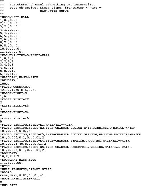
The input deck for the present example is shown in Figure 42. It is one of the examples in the CalculiX test suite. The channel is made up of six 3-node network elements (type D) in one long line. The nodes have fictitious coordinates. They do not enter the calculations, however, they will be listed in the .frd file. For a proper visualization with CalculiX GraphiX it may be advantageous to use the correct coordinates. As usual in networks, the final node of the entry and exit element have the label zero. The material is water and is characterized by its density, heat capacity and dynamic viscosity. Next, the elements are stored in appropriate sets (by using *ELSET) for the sake of referencing in the *FLUID SECTION card.

The structure of the channel becomes apparent when analyzing the *FLUID SECTION cards: upstream there is a sluice gate, downstream there is a large reservoir and both are connected by a straight channel. Like most upstream elements the sluice gate actually consists of two elements: the actual sluice gate element and a sluice opening element. This is because, although the gate fixes the water depth at its lower end, this water depth may be overrun by a backwater curve controlled by the downstream water level. The sluice gate is described by its width (10 $m$, which is constant along the channel), a slope of 0.005 (also constant along the channel) and a gate height of 0.8 $m$. Furthermore, the label of the downstream gate opening element has to be provided as well (3). The sluice opening element has the same width and slope, its length is 0.1 $m$. If a nonpositive length is provided, the true length is calculated from the nodal coordinates. The angle $\theta$ is zero, which means that the cross section is rectangular and not trapezoidal. Since the parameter MANNING has been used on the *FLUID SECTION card, the next parameter (0.01 $m^{-1/3}s$) is the Manning coefficient. Finally, the label of the upstream sluice gate element is given (2). The constants for the straight channel element can be checked in Section 6.5. Important here is the length of 49.8 $m$. The last element, the reservoir, is again a very short element (length 0.1 $m$). The length of elements such as the sluice opening or reservoir element, which do not really have a physical length, should be kept small.

Next, the boundary conditions are defined: the reservoir fluid depth is 2.7 $m$, whereas the mass flow is 60000 $kg/s$. Network calculations in CalculiX are a special case of steady state heat transfer calculations, therefore the *HEAT TRANSFER, STEADY STATE card is used. The prevailing force is gravity.

When running CalculiX a message appears that there is a hydraulic jump at relative location 0.67 in element 4 (the straight channel element). This is also clear in Figure 43, where the channel has been drawn to scale. The sluice gate is located at x=5 $m$, the reservoir starts at x=55 $m$. The bottom of the channel is shaded black. The water level behind the gate was not prescribed and is one of the results of the calculation: 3.667 $m$. The water level at the gate is controlled by its height of 0.8 $m$. A frontwater curve (i.e. a curve controlled by the upstream conditions - the gate) develops downstream and connects to a backwater curve (i.e. a curve controlled by the downstream conditions - the reservoir) by a hydraulic jump at a x-value of 38.5 $m$. In other words, the jump connects the upstream supercritical flow to the downstream subcritical flow. The critical depth is illustrated in the figure by a dashed line. It is the depth for which the Froude number is 1: critical flow.

In channel flow, the degrees of freedom for the mechanical displacements are reserved for the mass flow, the water depth and the critical depth, respectively. Therefore, the option U underneath the *NODE PRINT card will lead to exactly this information in the .dat file. The same information can be stored in the .frd file by selecting MF, DEPT and HCRI underneath the *NODE FILE card.