![]()
Evaluation of Existing Mass Distribution Model for
Multi-Orifice Flows
by
Jason Sydney Barnwell
Submitted to the Department of Mechanical Engineering
in Partial Fulfillment of the Requirements for the Degree of
Bachelor of Science
at the
Massachusetts Institute of Technology
January 2000
©2000 Massachusetts Institute of Technology
All rights reserved
Signature of Author
Department of Mechanical Engineering
January 14, 2000
Certified by
Jung-Hoon Chun
Associate Professor of Mechanical Engineering
Thesis Supervisor
Accepted by
Ernest G. Cravalho
Professor of Mechanical Engineering
Chairman, Undergraduate Thesis Committee
Evaluation of Existing Mass Distribution Model for
Multi-Orifice Sprays
by
Jason Barnwell
Submitted to the Department of Mechanical Engineering
On January 14, 2000, in partial fulfillment of the
Requirements for the degree of
Bachelor of Science in Mechanical Engineering
Evaluation of Existing Mass Distribution Model for
Multi-Orifice Flows
by
Jason Sydney Barnwell
Abstract
Droplet-Based Manufacturing (DBM) is an application of the Uniform Droplet Spray (UDS) process developed at the MIT Laboratory for Manufacturing and Productivity. DBM creates deposits using metal droplets that are generated at a consistent rate and size. These droplets can be collected in a specific pattern to produce a near-net-form end product or part. The quality of the end product is governed by the uniformity of the droplets and the ability to predict droplet behavior after droplet generation. Most of the research performed at MIT to date has focused on single jet sprays. Further development of this technology requires the use of multiple sprays to meet increasing mass flux requirements for various industrial applications.
In this research, an existing simulation model's ability to predict deposit geometry was evaluated for multiple jet sprays. This was accomplished by capturing deposits and comparing them to the output of the simulation. The existing model, developed by Godard Abel (Abel, 1993), has the capacity to predict droplet flight trajectory, thermal state, and deposition geometry. The model calculates droplet flight trajectory by summing the theoretical forces on the droplets the simulation generates, and the simulation tracks the location where the droplets land. This model is accurate for cases where the liquid metal jets are perfectly normal to the plane of the crucible bottom plate, but when an array of jets that are not normal to the crucible bottom plate is employed, the original simulation lacked the capacity to fully characterize the initial spray conditions.
Abel's simulation model was modified to allow for a more thorough characterization of the angular divergence of the initial jet trajectory with respect to the crucible bottom plate. The original simulation allowed axial variation from the normal vector of the crucible bottom plate as an angle of elevation, but only in one preset azimuthal direction. The modifications added a degree of freedom that permits initial trajectories with any angle of elevation and any azimuthal angle. The axial divergence for an orifice configuration was found empirically, and the simulation inputs were adjusted accordingly. The output of the modified simulation more accurately predicted the experimental deposit geometry.
Thesis Supervisor: Dr. Jung-Hoon Chun
Title: Associate Professor of Mechanical Engineering
Acknowledgements
I will be forever indebted to Professor Chun for his roles as mentor, advisor, and friend. His ability to teach with the allegory is both subtle and elegant. Jeanie Cherng took me under her wing in the lab and always had time to: question and answer; explain and obfuscate; argue and defend; chide and applaud; teach and learn. Ho-Young Kim gave me my first job in the DBM Lab and explained the UDS process to me, and for that I thank him. Wayne Hsiao is a truly selfless individual who repeatedly went out of his way to help me with my research, and life. Jiun-Yu Lai was always very graceful in giving up his lab key when research went deep into the night. Lisa Falco was a mooring post of sanity that provided us all with a firmer grasp on reality through her wit, charm, and humour. Karl Godard Abel's work is the basis of my research and I appreciate his competence and thoroughness. All of these individuals had direct impact on my research and will always remain beneficiaries of my gratitude.
My father and mother, Thomas and Susan Carter Barnwell, were the providers and benefactors during my entire MIT career. They were there for me always and in all ways. Thank you.
Table of Contents
Title Page 1
Abstract 2
Acknowledgements 3
Table of Contents 4
List of Figures 6
List of Tables 8
1. INTRODUCTION 9
1.1 Motivation and Background 9
1.2 Objectives 9
1.3 Overview of the Thesis 10
2. BACKGROUND 11
2.3 Droplet Flight Numerical Simulation 20
3.2 Spray Collection 24
3.3 Spray Deposit Analysis 25
4. RESULTS 27
5. SUMMARY 39
BIBLIOGRAPHY 41
APPENDIX A: Simulation Code 42
APPENDIX B: Simulation Input File 50
APPENDIX C: Experimental Data 51
List of Figures
Figure 2.1 Schematic of Uniform Droplet Spray System 11
Figure 2.2 Image of Spray Chamber and Experimental Control Panels 12
without UDS Crucible
Figure 2.3 Schematic of Uniform Droplet Spray Crucible 13
Figure 2.4 Images of : (a) Chamber Top Plate, 13
(b) Top Plate Inverted to show Crucible
Figure 2.5 Diagram of Charge Induction on Droplets during Jet Break-up 16
Figure 2.6 Diagram of Forces Acting on a Charged Droplet in Flight 18
Figure 3.1 Images of: Orifice Fixturing Options, (a) Caseless, 21
(b) Stainless Threaded, (c) Swaged Brass
Figure 3.2 Image of Orifice Jewels Fixtured In Brass 21
and Glued onto Graphite Crucible Bottom Plate
Figure 3.3 Image of Thread Fixtured Orifices Mounted in 22
a Stainless Steel Crucible Bottom Plate
Figure 3.4 Image of: (a) Crucible Bottom plate with Bottom Tapped Hole, 23
(b) Threaded-Stainless Steel Orifice Fixture
Figure 3.5 Image of Crucible Bottom Plate, Drilled and Tapped for 23
Thread Fixtured Orifices
Figure 3.6 Image of Spray Collection Grid with 5mm Square Cells 24
Figure 3.7 Image of Spray Collection Grid-Magnified View 25
Figure 4.1 Plots of: (a) Sum of Experimental Data Across Rows, 28
(b) Sum of Experimental Data Across Columns
Abscissa- Real Length Scale in Meters
Ordinate- Normalized Relative Height Scale
Figure 4.2 Contour Plots of: (a) Experiment 1, (b) Experiment 2 29
Abscissa and Ordinate- Real Length Scale in Meters
Normalized Relative Height Scale
Figure 4.3 Plots of Sum Across Rows for Experimental and 31
Simulation Data, (a) Experiment 1, (b) Experiment 2
Abscissa- Real Length Scale in Meters
Ordinate- Normalized Relative Height Scale
Figure 4.4 Plots of Sum Across Columns for Experimental and 31
Simulation Data, (a) Experiment 1, (b) Experiment 2
Abscissa- Real Length Scale in Meters
Ordinate- Normalized Relative Height Scale
Figure 4.5 Contour Plot for Simulation Data 32
Abscissa and Ordinate- Real Length Scale in Meters
Normalized Relative Height Scale
Figure 4.6 Large Spray Chamber with Computer Controlled-3 Axis Stage 33
Figure 4.7 Plot of Experimental Orifice Jet Trajectories with 33
Ideal Trajectory for Orifice # 3 Projected for Comparison
Figure 4.8 Diagram of Coordinate System Definition 34
Cartesian to Polar
Figure 4.9 Plots of Sum Across Rows for Experimental and 36
Modified-Simulation Data (a) Experiment 1, (b) Experiment 2
Abscissa- Real Length Scale in Meters
Ordinate- Normalized Relative Height Scale
Figure 4.10 Plots of Sum Across Columns for Experimental and 37
Modified-Simulation Data (a) Experiment 1, (b) Experiment 2
Abscissa- Real Length Scale in Meters
Ordinate- Normalized Relative Height Scale
Figure 4.11 Contour Plot of Modified Simulation Data 37
Abscissa and Ordinate- Real Length Scale in Meters
Normalized Relative Height Scale
List of Tables
Table 4.1 Experimental Parameters for Spray Tests 29
Table 4.2 Simulation Input Parameters 30
Table 4.3 Experimental Jet Trajectory Data 34
Table 4.4 Modified Simulation Input Parameters 35
Table C.1 Experimental Parameters for Data 51
Table C.2 Experiment One Data Array 52
Units: Milligrams
Scale: 5mm Square per Element
Table C.3 Experiment Two Data Array 52
Units: Milligrams
Scale: 5mm Square per Element
1 INTRODUCTION
1.1 Motivation and Background
Droplet-Based Manufacturing (DBM) uses metal droplets to form near-net-shaped deposits. DBM takes advantage of the Uniform Droplet Spray (UDS) process, which creates droplets of uniform size and thermal state (Chun et al., 1993). Ultimately, UDS improves the quality of processes that use DBM, because the uniformity of the droplets creates more reliably predicted final products.
Multi-orifice sprays represent a useful departure from single jet sprays because having a greater number of ports provides increased mass flux. Spraying a large sheet with a single spray jet requires the spray head to traverse a path that constructively uses spray edge effects to produce a flat deposit pattern (Lai, 1997). The disadvantage of this process is that successive sweeps result in disparate thermal states that create voids and irregular grain boundaries. These defects result in a deposit that can have segmented layering and can exhibit the effects of thermal creep and warping as the deposit cools unevenly. Multi-orifice arrays allow a larger spray to be created; the resulting deposit is more uniform in thermal state, so the bulk thermal effects resulting from disparate thermal states are reduced. By altering the initial temperature and flight distance, re-melt can take place on the substrate surface to produce a larger spray sheet with greater homogeneity. This specific potential of multi-orifice spraying promises future industrial use in spray forming/coating.
1.2
ObjectivesThere has been significant research done on many of the phenomena surrounding the UDS process and its ancillary technologies, but much of this research has focused on the issues involved in single jet sprays. There has been work done on manipulating a single jet spray to produce larger sheet effects (Lai, 1997), and the development of modeling techniques (Abel, 1993). The existing model can predict the behaviour of single orifice sprays, but little has been done to verify the existing model accuracy when multiple jets are used. Therefore, the scope of this research was to investigate the accuracy of this model when used to simulate multiple jets and to refine it if necessary.
This chapter provides an introduction to the project, its objectives, and a brief look at the motivation and background information concerning the UDS process and the modeling of multi-orifice sprays. Chapter 2 will provide some detail into the principles that the model uses to predict droplet flight. Chapter 3 will focus on the procedure and apparatus used to perform the experiments. Chapter 4 will present and discuss the specific experimental procedure and results. Finally, a summary of the thesis will be presented in Chapter 5.
2 BACKGROUND
2.1
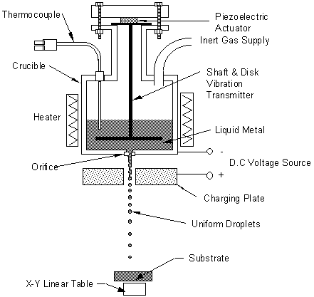
The UDS Process and EquipmentDroplet-Based Manufacturing (DBM) is built on the principle of depositing molten metal droplets. This process can be used in applications ranging from spray forming and rapid prototyping to electronic packaging. Notably, improving the quality of parts produced from DBM systems depends on improving control over the droplets produced by such systems. Such a system is a significant improvement over conventional gas-atomized processes because of the difficulty of dealing with droplets that vary in size and thermal state.
 The UDS system implements an apparatus designed to spray uniformly charged droplets, which all have consistent velocities and thermal histories (Passow, 1990). A diagram of the UDS apparatus is shown in Figure 2.1, and a photograph in Figure 2.2.
Figure 2.1 Schematic of Uniform Droplet Spray System

Figure 2.2 Image of Spray Chamber and Experimental Control Panels without UDS Crucible
The UDS system uses closed-loop control to power a resistance-type band heater. This heater is fitted around the crucible, and is used to supply the heat necessary to melt the metal to be sprayed. The temperature of the melt is monitored by a thermocouple inserted into the crucible. Many metals oxidize very rapidly when heated, so the crucible and spray chamber are filled with a chemically inert gas to abate this problem. Orifices are mounted on a plate mounted to the bottom of the crucible. Laminar jets are produced through these orifices by applying a gas pressure above the ambient chamber gauge pressure on the molten metal. A stack of piezoelectric crystals actuates the vibration rod that is placed within the crucible. Figure 2.3 shows a schematic representation of the UDS crucible, Figure 2.4(a) an image of the crucible and chamber top plate, and Figure 2.4(b) the chamber top plate and crucible inverted to show crucible detail.
Figure 2.3
Schematic of Uniform Droplet Spray Crucible

(a) (b)
Figure 2.4 Images of : (a) Spray Chamber Top Plate, (b) Top Plate Inverted to show Crucible
The vibration rod perturbs the melt at a specified frequency and transmits this vibration to the laminar jets ejected from the orifices. According to Rayleigh's theory of instability (Rayleigh,1878), jet perturbations at the appropriate frequency produce oscillations in the jet radius, which grow exponentially as they travel down the jet. These perturbations cause the laminar jet to break up into uniform droplets. A charging plate induces a charge on the droplets as they break from the jet. The charging plate has voltage potential, and when the laminar jet passes through the field, it picks up charge from the ground plate, (see Figure 2.5). This charge remains when the perturbations eventually cause the droplets to form. The droplets are all charged with the same polarity, and thus, repel each other. This induced charge prevents the droplets from merging in flight and causes them to form ring-shaped deposits. These droplets can then be either collected for use as powders, or deposited on a substrate.
2.2 Modeling of Droplet Flight to Substrate
The model that is evaluated in this thesis was developed by Godard Abel (Abel, 1993). His model was based on the physical principles governing motion for droplets in flight, coulombic interactions between droplets, and the thermal histories of the droplets as they fell. Based on this physical model, he developed a numerical computer simulation model that predicts the deposit resulting from the collection of a molten droplet spray. A general description of the modeling employed by Abel is described below.
2.2.1 Laminar Jet Break-up
When the molten metal is first ejected from the orifice, it consists of a continuous jet. The nature of this jet is that it is inherently, periodically unstable; that is, it can be broken into uniform droplets if a small perturbation is introduced into the jet. The first
stage of the droplet flight begins with this break-up of the laminar jet into individual droplets. This occurs when the perturbation generated by the vibration rod is at the proper frequency, see Figure 2.3. The Rayleigh frequency for the break-up of a laminar jet, fs, into uniform droplets is governed by the initial jet velocity , vj, and the jet diameter, dj:
 (2.1)
(2.1)
In this instance, the jet diameter is presumed to be equal to the orifice diameter. Uniform droplets should form when a laminar jet is perturbed at this frequency.
The initial velocity of the jet is governed by the following relationship, wherein Pdriving is the pressure difference between the crucible and the chamber, rl is the density of the liquid, and Cnoz is the discharge coefficient based empirically on the orifice size, the orifice shape, and the surface tension of the liquid (Passow, 1990):
 (2.2)
(2.2)
The droplet diameter, dd, is dependent upon the perturbation frequency, f, the mass flow rate, ![]() , and the density of the metal, r
m:
, and the density of the metal, r
m:
 (2.3)
(2.3)
2.2.2 Droplet Charging
To keep the droplets separated during the flight from the orifice to the substrate, a charge is induced upon the droplets as they exit the orifice and pass through a charging plate. As shown in Figure 2.5, the molten jet enters the charging plate as a continuous piece of molten metal. The jet is grounded, and as it passes through the field created by the voltage potential, a capacitance effect is created, and the jet picks up an induced charge. As the jet breaks up, the droplets retain the induced charge. The voltage potential is typically on the order of 1 kV.

Figure 2.5
Diagram of Charge Induction on Droplets during Jet Break-upThe amount of charge picked up by each droplet can be predicted by modeling the jet as a continuous line of charge with capacitance per unit of length.
The electrical field, E, surrounding a line of charge is given by (Cheng, 1983):
 (2.4)
(2.4)
where q' is charge per unit length, e o is the permattivity of free space, and r is the radial distance from the jet. The voltage potential, V, for a cylindrical capacitor is calculated by integrating the electrical field from the perimeter of the jet, dj, to the charging ring surface, dc:
 (2.5)
(2.5)
The charge per unit length, C', is equal to the charge, q', divided by the potential difference, V, and is equal to:
![]() (2.6)
(2.6)
For a cylindrical capacitor, the charge per unit length equals:
 (2.7)
(2.7)
The charge on each droplet is the charge per unit length multiplied by the droplet break-up wavelength:
![]() (2.8)
(2.8)
2.2.3 Droplet Flight Trajectory
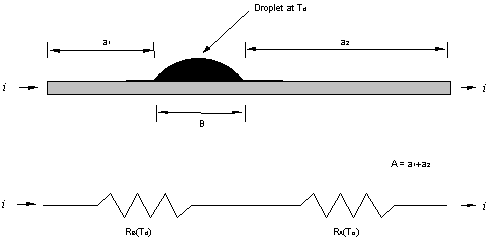
The flight of a droplet is dependent upon its initial velocity, Vd, the drag caused by its movement through the environment, Fd, the force resulting from gravity, Fg, and the force resulting from other charged droplets, Fc. The free body diagram, Figure 2.6, shows the forces acting on a droplet while in flight. The X, Y, and Z coordinate references made in subsequent equations are based on the coordinate system shown in Figure 2.6.

Figure 2.6
Diagram of the Forces Acting on a Charged Droplet in FlightThe resulting equation governing the motion of the droplet in free flight is:
 (2.9)
(2.9)
where, Vd, is the droplet velocity. The drag force acting on the droplet is:
 (2.10)
Where Cd is the drag coefficient, and the droplet material density is r m.
The drag coefficient for a droplet in flight is given by (Mathur, 1988):
![]() (2.11)
(2.11)
where Re is the Reynold's number for the given gas environment that has a viscosity, m g. The resulting Reynold's number is:
 (2.12)
The repulsion between like charged bodies is governed by coulombic force, so for the ith droplet the force created by the nearest n droplets is:
 (2.13)
where rij is the distance between droplets i and j.
The acceleration of droplet i in the X axis becomes:

 (2.14)
where D xij is the distance between droplets i and j. Similarly, the acceleration of droplet i in the Y axis is:

 (2.15)
where D yij is the distance between droplets i and j.
For the Z component a gravitational element is added:

where D zij is the distance between droplets i and j.
The simulation uses these equations of motion to model droplet flight as the droplets move from the orifices, to the substrate.
2.3 Droplet Flight Numerical Simulation
The numerical-simulation model that Abel created generates a finite number of droplets in the computer's memory. It then simulates the motion of said droplets to a prescribed final distance. The program records the final X,Y location of the droplets, and locates them within a rectangular grid system. Because each droplet is the same size, knowledge of the number of droplets that have landed in a particular grid square, will yield both the total mass that has landed in that square and the relative height of the total material in that square. The data that results from this modeling program is a 3-dimensional array; within this array are the respective numbers of droplets inside each element of an N x N matrix. Because the scale of each element, N, is known, the output can be mapped to a scale that represents real physical size. The simulation output can be normalized and resampled such that it can be compared to experimental data.
3 TESTING PROCEDURE
3.1.1 Orifice Fixturing and Mounting
The orifices that are used in spraying metals are typically ruby jewels that have been drilled to a nominal internal diameter. These materials are non-reactive and non-wetting for Sn alloys, and have excellent thermal and wear resistance properties. These jewels can be fabricated without any casing, Figure 3.1 (a), mounted in threaded stock made out of stainless steel, Figure 3.1 (b), or swaged into brass press fits, Figure 3.1 (c).


(a) (b) (c)
Figure 3.1 Images of: Orifice Fixturing Options, (a) Caseless,
(b) Stainless Threaded, (c) Swaged Brass
Previously, most orifices used in the DBM Laboratory were mounted in slip fit pockets within a crucible bottom, Figure 3.2.

Figure 3.2
Image of Orifice Jewels Fixtured In Brass, Glued onto Graphite Crucible Bottom PlateThe jewel orifice was held in place using high temperature glue. Replacing these orifices requires considerable skill, and improper mounting of a glued orifice can result in leaks around the outer edge of the orifice or in the ejection of the orifice during experimentation. Thread fixtured orifices, Figure 3.3, were integrated into this research because of the advantages they offer: decreased replacement time, increased leak resistance, and improved mounting consistency.

Figure 3.3
Image of Thread Fixtured Orifices Mounted in Crucible Bottom Plate3.1.2 Jet Stability
The UDS process works very well when the jet break-up is stable, but when the jets are not stable, the data collected in such experiments becomes unreliable. As more orifices are added to the array, it becomes increasingly difficult to maintain stability in all of the jets. Balancing the jets adds more non-useable spraying time, but this stability is necessary for the data to be valid. Increasing the number of orifices increases the mass flux; this reduces the time in which experiments can be debugged and run, because the crucible holds a finite amount of spray material. Using concurrent jets depletes the molten metal reservoir more rapidly.
When a single jet is sprayed, small variations in the initial jet velocity are not very noticeable. When an array of jets is sprayed, however, they are significantly close, and consequently small angle deflections are very noticeable in relation to the other jets. These initial deflections make it more difficult to predict the deposit structure and thus, the simulation becomes less reliable. The threaded orifices reduced the initial velocity differences caused by mounting inconsistencies, Figure 3.4 (b).

(a) (b)
Figure 3.4
Image of: (a) Crucible Bottom plate with Bottom Tapped Hole,(b) Threaded-Stainless Steel Orifice Fixture
Using threaded orifices does increase the complexity of the bottom plate, which requires precision bottom-tapped threads, Figure 3.5.

Figure 3.5
Image of Crucible Bottom Plate, Drilled and Tapped for Thread Fixtured OrificesJet stability is also affected by jewel surface quality, material oxidation, atmospheric cleanliness, and perturbation intensity (Yim, 1996). Small blockages or trace amounts of oxygen in the chamber environment can significantly hinder jet stability and can prevent consistent break-up.
The evaluation of the existing model requires comparison between numerically simulated and experimental results. This was accomplished by creating a metal grid in which to collect the deposit. A piece of .25'' thick Aluminum plate was machined using a waterjet and was then cut to form a 29 x 29 grid of 5 mm squares, Figure 3.6.
Figure 3.6
Image of Spray Collection Grid with 5mm Square CellsThe grid was placed at the bottom of the chamber, and centered beneath the crucible bottom plate. When the metal was sprayed in the chamber, deposit accumulated in the individual grid cells. The superheat of the melt was set at 18o C above the melting temperature of the spray material, Sn- melting temperature 232o C, to ensure that almost fully solidified droplets filled the grid, Figure 3.8. As can be seen in the magnified view of the collection grid shown in Figure 3.7, the majority of the spray landed in the discrete cells, with very little remaining on the vertical dividers.
Figure 3.7
Image of Spray Collection Grid-Magnified ViewThis consideration to melt temperature reduced the mushrooming effect that occurs when molten metals strike cold, finned surfaces. Mushrooming occurs when the molten droplets rapidly solidify on the leading edges, blocking the entries to the cells as the metal deposit blossoms outward.
After the spraying was complete, the grid was removed from the spray chamber and the deposit from each grid square was extracted and weighed. The mass from each cell was recorded along with a grid coordinate reference corresponding to its location, referenced from the bottom left corner of the collection grid. A Mettler AT20 scale was used to mass the sections of the deposit. The mass data was recorded in milligrams: the AT20 has a deviation of +/- 2 mg.
The resulting N x N array of masses could be manipulated in the same ways as the output of the modeling program. The analysis of the data required normalization between the experimental data sets and the simulation data sets. This entailed putting the outputs of both data sets into the same units of measure. The X and Y scale of the experimental data corresponded to the spacing of the cells in the collection grid, with each cell measuring 5mm square. The X and Y scale of the simulation is calculated in the modeling process and was generated as a separate file at the conclusion of the simulation. Dividing each mass element of the experimental data array by the mass of the total array generated a new array with a Z scale of non-dimensionalized height. For the simulations, dividing the number of droplets in each array element by the sum of all the droplets in the array created a new array that also had a Z scale of non-dimensionalized height. The resulting data sets had comparable scales that were centered on the same origin, relative to the deposits, and could be visually compared for geometric similarity. The raw experimental data can be found in Appendix C. The code for simulation can be found in Appendix A.
4 RESULTS
4.1 Experimental Data
Obtaining the experimental data involved many steps. First, the crucible had to be prepared. This involved: loading the melt material, Sn 100%, into the crucible; bolting the crucible bottom plate to the crucible; bolting the charging plate and insulators to the crucible bottom plate; and affixing the voltage lead to the charging plate. After the crucible was prepared, the collection grid had to be readied. Preparation included: applying spray adhesive to the back of the collection grid; adhering aluminum foil to the back of the collection grid; and placing the grid on a pedestal within the spray chamber. After the crucible and collection grid were ready, a moveable collection cup was fitted under the chamber top plate that holds the crucible. The cup sat underneath the crucible bottom plate and was used to collect the spray not intended for the collection grid. The whole assembly was placed on top of the chamber through its top opening and bolted to the upper chamber flange.
After the top plate was attached and the gas supply lines were engaged to their respective ports, the chamber was atmospherically sealed. At that point, the chamber was vacuumed to 200 hundred millitorr, and then filled to 5 psi gauge, with Nitrogen. This vacuuming and filling process was repeated again, and after the second filling procedure, the heater was turned on and the crucible was brought to a stable 250o C. The signal generator was turned on and the crucible was pressurized to 20 psi, gauge. The jets could be seen from an observing camera, and when they had stabilized, the amplifier that supplies voltage to the charging plate was turned on and set for 1500 volts. The collection cup was then moved out of the way, and the collection grid was sprayed until the cells that had collected the most material were nearly full. The collection cup was swung back under the jets and the spraying was halted. All the equipment was shut down, the gas supplies turned off, and the top plate removed to allow access to the chamber. Once the collection grid was removed, the deposit analysis process, outlined in section 3.3, was employed.
The experimental data that was gathered is shown graphically in Figures 4.1 and 4.2. Figure 4.1 shows the normalized data summed across rows in (a), and across columns in (b). The plots of Figure 4.1 show what the deposit geometry would look like if the substrate were swept relative to the spray across the rows, i.e. parallel to the X axis, Figure 4.1(a), and across the columns, i.e. parallel to the Y axis, Figure 4.1(b). These plots are effectively the cross sections of a sheet sprayed using this experimental set up. The plots also show great similarity between the two data sets in relative scale and the position of peaks.
(a) (b)
Figure 4.1 Plots of: (a) Sum of Experimental Data Across Rows,
(b) Sum of Experimental Data Across Columns
The contour plots, 4.2(a) and 4.2(b), show the topology of a static spray, that is, the substrate does not move relative to the spray. On contour plots, regions of equal relative height are shown by a contour line. Contours that are closer together represent a steeper rise in elevation. On the plots in Figure 4.2, there is some variation in the deposit geometry due to experimental deviation, but the three, ring-shaped deposits on each plot are centered in very similar relative locations. The consistency of the two data sets suggests that they are reproducible.
(a) (b)
Figure 4.2 Contour Plots of: (a) Experiment 1, (b) Experiment 2
Both experiments were performed under the same parameters, Table 4.1.
Table 4.1
Experimental Parameters for Spray Tests|
Parameter |
Experiment 1 |
Experiment2 |
|
Spray Material |
100% Sn |
100% Sn |
|
Driving Pressure |
20 psi gauge |
20 psi gauge |
|
Driving Frequency |
3.4 kHz |
3.4 kHz |
|
Droplet Charging |
1.5kV |
1.5kV |
|
Charging Slot Width |
1.27 cm |
1.27 cm |
|
Melt Temperature |
250o C |
250o C |
|
Flight Distance |
79 cm |
79 cm |
|
Orifice Diameter |
200 micron |
200 micron |
|
Orifice Position 1 (x,y)* |
-4.30 mm, 2.48 mm |
-4.30 mm, 2.48 mm |
|
Orifice Position 2 (x,y)* |
-4.30 mm,-2.48 mm |
-4.30 mm,-2.48 mm |
|
Orifice Position 3 (x,y)* |
4.96 mm, 0.0 mm |
4.96 mm, 0.0 mm |
*
positions measured from geometric center of orifice bottom plate
4.2 Simulation Data
A comparison of experimental data with data from the simulation is shown in Figures 4.3(a), 4.3(b), 4.4(a), 4.4(b); these plots are of the same type as those in Figure 4.1. The plots in Figure 4.3 compare the simulation data and experimental data, summed across rows, and the plots in Figure 4.4 compare the simulation data and experimental data summed across columns. The parameters that were input into the simulation were identical to those used in the experiments, Table 4.2.
Table 4.2
Simulation Input Parameters|
Parameter |
Simulation |
|
Spray Material |
100% Sn |
|
Driving Pressure |
20 psi gauge |
|
Driving Frequency |
3.4 kHz |
|
Droplet Charging |
1.5kV |
|
Charging Slot Width |
1.27 cm |
|
Melt Temperature |
250o C |
|
Flight Distance |
79 cm |
|
Orifice Diameter |
200 micron |
|
Orifice Position 1 (x,y) |
-4.30 mm, 2.48 mm |
|
Orifice Position 2 (x,y) |
-4.30 mm,-2.48 mm |
|
Orifice Position 3 (x,y) |
4.96 mm, 0.0 mm |
It can be qualitatively seen in Figures 4.3(a), 4.3(b), 4.4(a), and 4.4(b) that the peaks do not match well in location and number. The overall width of the simulated deposits is much larger than the experimental deposits. These differences were consistently observed when the simulation was employed.
(a) (b)
Figure 4.3
Plots of Sum Across Rows for Experimental and Simulation Data(a) Experiment 1, (b) Experiment 2
(a) (b)
Figure 4.4 Plots of Sum Across Columns for Experimental and Simulation Data
(a) Experiment 1, (b) Experiment 2
The disparity between the simulation and the experimental data is further emphasized when the contour plots for the experimental data, Figures 4.2 (a) and (b), are compared to the contour plot for the simulation, Figure 4.5.

Figure 4.5
Contour Plot for Simulation DataThe experimental contour plots showed 3 nearly discrete regions with a distinctive asymmetry, while the simulation predicted a very symmetric geometry. Additionally, the simulation exhibits constructive interference on the boundaries, where the sprays overlap and form one large, continuous mass, rather than 3 separate rings.
4.3 Jet Axial Divergence
Comparing the experimental data and the simulation results revealed a significant discrepancy. Further investigation suggested that one of the orifices mounted on the crucible bottom plate was consistently creating an axially divergent jet. Initially, it was believed that the orifice jewel, or the thread fixture that the jewel mates to, was faulty and that replacing the unit would solve the problem. However, further trials revealed that the problem was not solved after the orifice unit was replaced, and that in fact, the same orifice position on the bottom plate was exhibiting similar off-center jet trajectory. This implied that the problem existed in the crucible bottom plate, which held the thread-fixtured orifices. The consistency of the off-center spray was most likely due to the improper tapping of the bottom plate during the machining process. The orifices may deviate from the normal plane of the crucible bottom plate very little, but for spraying over longer spray distances, this deviation can be significant.
An experiment to measure this deviation was set up using a 3-axis, moveable stage installed in a large spray chamber, Figure 4.6.

Figure 4.6
Large Spray Chamber with Computer Controlled-3 Axis StageUncharged jets were sprayed onto a room temperature aluminum substrate, 54 cm below the crucible bottom plate. The jets formed small circular globules, approximately 5 mm in diameter, where they impacted the substrate. The stage was lowered 21 cm and translated laterally 6 cm. Again, the jets were used to create 3 more small globules. The positions of these globules were then used to extrapolate the jet trajectories, and the amount of axial divergence for each jet, Figure 4.7.

Figure 4.7
Plot of Experimental Orifice Jet Trajectories with Ideal Trajectory for Orifice # 3 Projected for ComparisonThe jet trajectory divergence was translated from Cartesian coordinates to polar coordinates, Figure 4.8.

Figure 4.8
Coordinate System Translation from Cartesian to PolarThe resulting deviation for each orifice is shown in Table 4.3.
Table 4.3
Experimental Jet Trajectory Data|
Orifice Number |
Position (X,Y) mm |
Elevation ( Q) degrees |
Azimuth ( F) degrees |
|
1 |
(-4.3, 2.5) |
0 |
0 |
|
2 |
(-4.3, 2.5) |
0 |
0 |
|
3 |
(5.0, 0.0) |
2 |
33 |
This divergence was believed to be the source of the variation between the original simulations and the experimental data. This experiment yielded a quantitative value for the amount of axial divergence for orifice 3.
4.4 Modified Simulation
Once quantitative values for the amount of axial divergence of each orifice position had been found, it was possible to alter the simulation to take this axial divergence into account. Abel’s simulation model had the capacity to create an initial angular displacement, but only within the X-Z plane. His simulation was changed to allow any orifice position to be given an initial trajectory of any vector within the lower hemisphere of XYZ space. The modified code can be found in Appendix A. The modified coordinate system, used in the modified simulation-model, is shown in Figure 4.8. In addition to the simulation's existing angle of elevation, Q, from axis Z in the Z-X plane, the degree of freedom about the Z axis, F, was added to the simulation.
The results of the modified simulation and experimental data are compared in Figures 4.9 (a), 4.9 (b) 4.10 (a), and 4.10 (b). Figures 4.9 (a) and (b) show the comparison of the experimental data and the modified-simulation data, summed across the data rows, as in Figures 4.3 (a) and (b). Figures 4.10 (a) and (b) show the comparison of the experimental data to the modified-simulation data summed across data columns, as in Figure 4.4s (a) and (b). The input parameters for the simulation are shown in Table 4.4.
Table 4.4
Modified Simulation Input Parameters|
Parameter |
Simulation |
|
Spray Material |
100% Sn |
|
Driving Pressure |
20 psi gauge |
|
Driving Frequency |
3.4 kHz |
|
Droplet Charging |
1.5kV |
|
Charging Slot Width |
1.27 cm |
|
Melt Temperature |
250o C |
|
Flight Distance |
79 cm |
|
Orifice Diameter |
200 micron |
|
Orifice Position 1 (x,y) |
-4.30 mm, 2.48 mm |
|
Orifice Position 2 (x,y) |
-4.30 mm,-2.48 mm |
|
Orifice Position 3 (x,y) |
4.96 mm, 0.0 mm |
|
Jet Divergence 1 (Q,F) |
0 o, 0 o |
|
Jet Divergence 2 (Q,F) |
0 o, 0 o |
|
Jet Divergence 3 (Q,F) |
2 o, 33 o |
In plots 4.9-4.10, the abscissa represents a real length scale, and the ordinate represents a relative height scale, normalized to 1.0. Figures 4.9-4.10 show a much closer mapping of scale and geometry between the experimental data and the modified-simulation data, when compared to the comparison plots of the experimental data and simulation, Figures 4.3-4.4.


Figure 4.9
Plots of Sum Across Rows for Experimental and Modified-Simulation Data(a) Experiment 1, (b) Experiment 2


Figure 4.10 Plots of Sum Across Columns for Experimental and Modified-Simulation Data
(a) Experiment 1, (b) Experiment 2
The contour plot for the modified simulation, Figure 4.11, also shows much greater geometric similarity to the contour plot for the experimental data, Figure 4.2 (a) and (b), than the contour plot for the simulation, Figure 4.5.

Figure 4.11
Contour Plot of the Modified-Simulation DataLike the experimental-data contour plots, the modified-simulation contour plot shows three distinct ring structures and the asymmetric positioning characteristic of the experimental data. The modified simulation maps well to the experimental data, and makes a prediction that is more consistent in the location of features, boundary effects and overall size. The modified simulation more accurately predicts the deposits for charged-droplet, molten-metal sprays that emanate from multiple jet arrays with axial divergence from the normal plane of the crucible bottom plate.
5 SUMMARY
Abel's modeling of charged UDS deposits was insufficient for cases where jets exhibit axial divergence from the normal plane of the crucible bottom plate, in which the orifices were mounted. His simulation can model the deposit topology and scale for the ideal case of jet trajectories perfectly normal to the plane of the crucible bottom plate. The modification made to Abel's code for the purpose of this research adds further flexibility to the simulation. His simulation can now be used for off-center jets of almost any configuration, however, this does require empirical determination of the orifices' axial divergence, with respect to angular displacement from the vector normal to the crucible bottom plate. This orifice configuration measurement can be accomplished with a CMM that uses a very small probe, or can be determined experimentally by analyzing deposits taken at precisely known relative positions.
Much of the difficulty involved in utilizing multiple orifice arrays in UDS applications will be due to the difficulty of orifice mounting. Small deviations of the jets from the normal vector of the mounting plane can create significant variation in the resulting spray patterns when compared to the expected spray deposits for squarely mounted orifices. If orifices and their resulting jets are not normal to the crucible bottom plate, then measures can be taken to mitigate the effect of the off-center jets on the resulting spray. The spray conditions can be altered such that the resulting deposit will more closely resemble the geometry of a spray deposit created using jets with trajectories normal to the crucible bottom plate. Minimizing the distance between the substrate and the spray head limits the distance the droplets travel, and consequently reduces the droplet drift in the X-Y plane. This does not reduce the jet’s angle of deflection, but it does decrease the amount of translation in the X-Y plane by reducing the hypotenuse length of the solid angle. Decreasing the pressure difference between the spray chamber pressure and the driving pressure yields similar results: the decrease in initial velocity reduces the velocity component of the droplet in the X-Y plane and mitigates the existing initial trajectory of the droplet's flight path. These techniques can result in changed thermal properties when the droplets strike the substrate, so the melt temperature or substrate temperature should be changed accordingly.
BIBLIOGRAPHY
Abel, Godard Karl. 1993. "Characterization of Droplet Flight Path and Mass Flux in Droplet-Based Manufacturing." S.M. Thesis. Massachusetts Institute of Technology.
Avallone , E.A. and T Baumeister, eds. 1987. Mark's Standard Handbook for Mechanincal Engineers. McGraw-Hill Book Company. New York.
Bechwith, T.G., R.D. Marangoni and J.H. Lienhard. 1995. Mechanical Measurements. Addison-Wesley Publishing Company. Reading, MA.
Cheng. 1983. Field and Wave Electromagnetics. Addison-Wesley Publishing Company. Reading, MA.
Chun, Jung-Hoon and C.H. Passow. 1991. "Production of Charged Uniformly Sized Metal Droplets." United States Patent # 5,266,098, November 30, 1993.
Deitel, H.M. and P.J. Deitel. 1999. Java How To Program. Prentice Hall. Upper Saddle River, NJ.
DeWitt, F.P. and D. P. Incropera. 1996. Fundamentals of Heat and Mass Transfer. John Wiley & Sons Inc. New York, NY.
Lai, Jiun Yu. 1997. "A Study of the Fabrication of Thin Lamination Stator Cores by the Uniform Droplet Spray Process." S.M. Thesis. Massachusetts Institute of Technology.
Mathur, P.C. 1988. "Analysis of the Spray Deposition Process." Ph.D. Thesis. Drexel University.
Pasachoff, J.M and R Wolfson. 1995. Physics for Scientists and Engineers. Harper Collins College Publishers. New York, NY.
Passow, Christian H. 1992. "A Study of Spray Forming Using Uniform Droplet Sprays." S.M. Thesis. Massachusetts Institute of Technology.
Rayleigh, F.R.S. 1878. "On the Instability of Jets." Proceedings of the London Mathematic Society. 10 (4):4-13.
Yim, Pyongwon. 1996. "The Role of Surface Oxidation in the Break-Up of Laminar Liquid Metal Jets." Ph.D. Thesis. Massachusetts Institute of Technology.
Appendix A SIMULATION CODE
The following code models the deposit geometry, and thermal history for charged UDS applications. Compile it in either the C or C++ programming languages. It was altered from an existing program to allow for greater control of initial jet conditions, specifically the initial axial divergence from the normal vector of the plane in which any given jet originates.
/*Godard K Abel-uniform charged metal droplet trajectories*/
/*program to predict single orifice droplet flight path*/
/*18.c-same as 16.c but it adds heat transfer correction*/
//This program was altered by Jason Barnwell 1/10/2000
//It now accepts 2 angles for each orifice to establish
//an initial trajectory vector, one from the Z axis , and another
//around the Z axis in the X-Y plane
//The end of the input file now takes 4 tab delimited values
//where the values are xpos ypos elevation azimuth
#include<stdio.h>
#include<math.h>
#include<stdlib.h>
FILE *inp; /*open file for inputs*/
FILE *dro; /*file to store drop velocity,temperature,enthalpy*/
FILE *res; /*open file for results*/
FILE *his; /*open file for histogram*/
FILE *cut; /*file for radial heigth distribution*/
FILE *gri; /*file for 3d mesh plot*/
FILE *ngr; /*file for numerical distribution grid*/
FILE *ndr; /*file for number of drops per section*/
FILE *spr; /*file to find spread angle of spray*/
FILE *mov; /*file to record shape of moving deposit*/
FILE *amv; /*file to record averaged shape of moving deposit*/
/*constants defined as global variables*/
double g=9.81; /*gravity (m/s^2)*/
double knitrogen=.0259; /*conductivity at 300K (Wq/m-K)*/
double pnitrogen=1.1233; /*density of nitrogen at 300K (kg/m^3)*/
double unitrogen=17.84e-6; /*viscosity of nitrogen at 300K (kg/ m-s)*/
double cnitrogen=1041; /*specific heat of nitrogen at 300K (J/kgK*/
double Pr=.715; /*Prandtl number for Nitrogen at 300K*/
double Tgas=27; /*chamber gas temperature (Celsius)*/
double e0=8.85e-12; /*permitivitty of free space*/
double cmsolid,cmliquid,Ts,pmetal,hof; /*metal/alloy properties*/
double xmin,xmax,ymin,ymax,rmax;
double **current;
/*initialize calculated constants as global variables*/
double distance,md,c1,cre,ccoul,d,f;
double e,temp;
int dif=0; /*number of droplets in flight*/
int nd=0; /*number of droplets created*/
int count=0; /*flag for when first drop reaches substrate*/
int old = 0;
int nn,norf,mp,N,deposited;
/*function prototypes*/
void runge_kutta(int,double **,
double(*)(double,double,double,double,double,double,int,double **,double),
double(*)(double,double,double,double,double,double,int,double **,double),
double(*)(double,double,double,double,double,double,int,double **,double,double,double),double);
double uprime(double,double,double,double,double,double,int,double **,double);
double vprime(double,double,double,double,double,double,int,double **,double);
double wprime(double,double,double,double,double,double,int,double **,double,double,double);
void thermal_state(double **,double,double);
void spread(double **,int);
void output(int,double **);
void histogram(int,double **);
void rcut(int,double **);
void grid(int,double **,int,double,double);
main()
{
double x=0; double y=0;
double pressure,od,runtime,volt, width, l; /*initialize inputs*/
double qd,capacitance,v0,level;
double h;
double t=0;
double kj;
int td,alloy,step;
int spd,i,k,n,c,j,jcra;
double **a;
double **orf;
int passes;
double disturbance;
double totalmass,speed;
double timed=0; /*time droplets depositing on substrate*/
/*dynamically allocate memory for array to store orifice positions*/
//orf=calloc(norf,sizeof(double *));
//for(i=0;i<norf;i++){
// orf[i]=calloc(2,sizeof(double));
//}
/*read inputs here from "inputs" file*/
inp=fopen("inputs","r");
fscanf(inp,"%d\n",&alloy); /*alloy number*/
fscanf(inp,"%lf\n",&temp); /*melt temperature*/
fscanf(inp,"%lf\n",&pressure); /*driving pressure (psi)*/
fscanf(inp,"%lf\n", &od); /*orifice diameter (m)*/
fscanf(inp,"%lf\n",&f); /*piezo-electric frequency (Hz)*/
fscanf(inp,"%lf\n",&width); /*width of charging slot (inches)*/
fscanf(inp,"%lf\n",&volt); /*charging plate voltage (V)*/
fscanf(inp,"%lf\n",&distance); /*distance from nozzle to substrate (m)*/
fscanf(inp,"%d\n",&td); /*total drops deposited*/
fscanf(inp,"%d\n", &spd); /*calculation steps per drop creation*/
fscanf(inp,"%d\n", &passes); /*number of passes depositing onto substrate*/
fscanf(inp,"%lf\n",&speed); /*speed of substrate (m/s)*/
fscanf(inp,"%lf\n", &disturbance);/*magnitude of disturbance*/
fscanf(inp,"%d\n",&nn); /*# of droplets in Coulomb force calculation*/
fscanf(inp,"%d\n\n",&N); /*# of elements in mass flux grid*/
fscanf(inp,"%d\n", &norf); /*number of orifices*/
nn=nn*norf;
/*dynamically allocate memory for array to store orifice positions*/
orf=calloc(norf,sizeof(double *));
for(i=0;i<norf;i++){
orf[i]=calloc(4,sizeof(double));
}
/*read orifice positions from file*/
for(i=0;i<norf;i++){
fscanf(inp,"%lf\t",&orf[i][0]); /*x-position of orfice*/
fscanf(inp,"%lf\t",&orf[i][1]); /*y-position of orifice*/
fscanf(inp,"%lf\t",&orf[i][2]); /*angle of orifice from z axis*/
fscanf(inp,"%lf\n",&orf[i][3]); /*angle of orifice around z axis ref from x axis*/
}
fclose(inp);
/*print orifice positions*/
printf("\nORIFICE POSITIONS\n");
for(i=0;i<norf;i++){
j=i+1;
printf("\nx-position of orfice # %d= %lf (m)\ty-position of orifice # %d= %lf (m)",
j,orf[i][0],j,orf[i][1]);
if(orf[i][2]!=0)
printf("\nangle from z axis of orfice # %d= %lf degrees\n",j,orf[i][2]);
printf("\nangle around z axis of orfice # %d= %lf degrees\n",j,orf[i][3]);
}
for(i=0;i<norf;i++){
orf[i][2]=orf[i][2]/180*3.142;
orf[i][3]=orf[i][3]/180*3.142;/*convert degrees to radians*/
}
dro=fopen("drop","w"); /*create files to be appended*/
fclose(dro);
spr=fopen("spread","w");
fclose(spr);
if(td<(20*norf)) /*make sure there are enough drops to track veloctiy and thermal state*/
td=20*norf;
if(norf>1)
td=((td/norf)+1)*norf;
mp=td/2; /*track around this particle*/
/*print inputs to simulation*/
printf("THE INPUTS TO THE SIMULATION:\n");
printf("melt temperature= %lf degress Celsius\talloy #%d \n",temp,alloy);
printf("driving pressure = %f psi\torifice diameter= %e m\n",pressure,od);
printf("piezo-electric frequency= %lf (Hz)\tcharge plate width= %e in\n",f,width);
printf("charging voltage= %f V \t\tflight distance= %f m\n",volt,distance);
printf("total # of drops= %d \t\t\tcalculation steps per drop= %d\n",td,spd);
printf("number of passes= %d\t\t\tsubstrate speed= %lf (m/s)\n",passes,speed);
printf("size of disturbance= %e x droplet diameter\n",disturbance);
printf("number of neighbors in coulomb force calculation= %d\n",nn);
if(alloy==1){
pmetal=9114; /*density of eutectic tin-37%lead (kg/m^3)*/
Ts=184; /*solidification temperature (Celsius)*/
cmliquid=216.7; /*specific heat of molten metal(J/kgK)*/
cmsolid=203.8; /*specific heat of solid metal(J/kgK)*/
hof=46054; /*heat of fusion of metal (J/kg)*/
}
if(alloy==2){
pmetal=7800; /*density of pure tin (kg/m^3)*/
Ts=232; /*solidification temperature (Celsius)*/
cmliquid=257.3; /*specific heat of molten metal(J/kgK)*/
cmsolid=244.4; /*specific heat of solid metal(J/kgK)*/
hof=59570; /*heat of fusion of metal (J/kg)*/
}
if(alloy==3){
pmetal=11350; /*density of pure lead (kg/m^3)*/
Ts=327.5; /*solidification temperature (Celsius)*/
cmliquid=147.5; /*specific heat of molten metal(J/kgK)*/
cmsolid=134.6; /*specific heat of solid metal(J/kgK)*/
hof=23040; /*heat of fusion of metal (J/kg)*/
}
if(alloy==4){
pmetal=7978; /*density of tin-5%lead (kg/m^3)*/
Ts=200; /*solidification temperature (Celsius)*/
cmliquid=251.8; /*specific heat of molten metal(J/kgK)*/
cmsolid=238.9; /*specific heat of solid metal(J/kgK)*/
hof=58894; /*heat of fusion of metal (J/kg)*/
}
if(alloy==5){
pmetal=9220; /*density of tin-40%lead (kg/m^3)*/
Ts=190; /*solidification temperature (Celsius)*/
cmliquid=213.4; /*specific heat of molten metal(J/kgK)*/
cmsolid=200.48; /*specific heat of solid metal(J/kgK)*/
hof=44958; /*heat of fusion of metal (J/kg)*/
}
/*calculate initial jet velocity*/
kj=1.0;
if(od>375e-6&&od<425e-6)
kj=.97; /*guesstimated orifice coefficient*/
if(od>90e-6&&od<110e-6)
kj=1.1547*sqrt(1.1); /*orifice coefficient for nominal 100um orifice*/
if(od<60e-6&&od>40e-6)
kj=1.1859; /*orifice coefficient for nominal 50um orfice*/
v0=kj*sqrt(pressure);
/*calculate droplet diameter*/
d=pow((1.5*pow(od,2.0)*v0/f),(1.0/3.0));
/*calculate droplet mass*/
md=(1.0/6.0)*3.142*(pow(d,3.0))*pmetal;
/*calculate initial droplet enthalpy*/
e=md*(((temp-Ts)*cmliquid)+(hof)+((Ts-Tgas)*cmsolid));
/*constant for calculating drag force*/
c1=.125*3.14*pnitrogen*d*d;
cre=pnitrogen*d/unitrogen; /*constant for calulating the reynold's number*/
/*calulate charge per droplet*/
l=v0/f; /*length of jet that forms each doplet=jet velocity/frequency*/
/*capacitance between jet and charging plate*/
width=width*.0254; /*convert inches to meters*/
capacitance=2.0*3.1416*e0*l/(.23+log(width/od));
//qd=4.5e-11;
qd=capacitance*volt; /*charge per droplet*/
/*constant for calculating the coulomb force between droplets*/
ccoul=qd*qd/(4*3.14*e0);
/*calculate integration increment in seconds*/
h=1/(f*spd);
/*print calculated constants here*/
printf("\nTHE PARAMETERS AND CONSTANTS CALCULATED FROM THE INPUTS\n");
printf("initial jet velocity=%lf (m/s) droplet diameter= %e (m) \n",v0,d);
printf("droplet mass = %e (kg)\n",md);
printf("drag constant c1= %e Reynold's constant= %f\n",c1,cre);
printf("jet length/drop= %e (m) capacitance= %e (F)\n",l,capacitance);
printf("charge per drop= %e (C) coulomb force constant= %e\n",qd,ccoul);
printf("integration step size= %e",h);
/*dynamically allocate memory for array to store droplet position+velocity*/
a=calloc(td,sizeof(double *));
for(i=0;i<td;i++){
a[i]=calloc(6,sizeof(double));
}
current=calloc(td,sizeof(double *));
for(i=0;i<td;i++){
current[i]=calloc(6,sizeof(double));
}
/*loop to create droplets and calculate droplet trajectories*/
dif=0;
step=0;
level=distance/50;
while(deposited<(td-norf+1))
//while(deposited<1000)
{ /*continue running until all drops reach substrate*/
// for (jcra=0;jcra<1000;jcra++){
if(nd<(td-(norf-1))) /*create drops until all are created*/
{
for(k=0;k<norf;k++) /*create droplets with random disturbance in this loop*/
{
a[nd][0]=orf[k][0]+(disturbance*d*(.5-rand()*1.0/RAND_MAX)); /*x-position*/
a[nd][1]=orf[k][1]+(disturbance*d*(.5-rand()*1.0/RAND_MAX)); /*y-position*/
a[nd][2]=0; /*initial z-position*/
a[nd][3]=sin(orf[k][2])*cos(orf[k][3])*v0; /*initial x-velocity*/
a[nd][4]=sin(orf[k][2])*sin(orf[k][3])*v0; /*inital y=velocity*/
a[nd][5]=cos(orf[k][2])*v0; /*initial z-velocity*/
nd+=1; /*keep track of total droplets created*/
dif+=1; /*keep track of number of droplets in flight*/
}
}
for(j=0;j<spd;j++) /*do this many calculations between droplet creations*/
{
if(count==1)
timed+=h;
for(i=nd;i>nd-dif;i--) /*store current position of droplets before*/
{ /*runge-kutta steps*/
for(k=0;k<6;k++)
{
current[i-1][k]=a[i-1][k];
}
}
if(a[mp][2]>level)
{
spread(a,td);
level+=distance/50;
}
if(nd>mp+1)
{
thermal_state(a,h,Tgas);
}
for(c=1;c<(dif+1);c++) /*for each drop in flight use runge kutta*/
{
n=nd-c;
runge_kutta(n,a,uprime,vprime,wprime,h);
}
}
step+=1;
printf("\nstep= %d, nd= %d, zmin= %lf,deposited=%d,td=%d,distance=%1f,level=%1f ",step,nd,a[mp][2],deposited,td,distance,level);
}
/*call output formatting functions here after completing simulation*/
output(td,a); /*print results to output file*/
if(norf==1)
rcut(td,a); /*radial cross-section of deposit*/
grid(td,a,passes,speed,timed);/*3D shape of deposit and moving cross-section*/
/*print important simulation results*/
printf("\n\nSIMULATION RESULTS\n");
runtime=spd*step*h;
printf("\nSimulation time= %lf\n",runtime);
printf("\nxmin= %lf xmax=%lf\n",xmin,xmax);
printf("\nymin= %lf ymax=%lf\n",ymin,ymax);
printf("\nrmax= %lf\n",rmax);
//deposited=td-dif; /*total number of droplets that reach substrate*/
printf("\ntotal number of droplets deposited= %d\t",deposited);
//totalmass=deposited*md*1000; /*total mass deposited in grams*/
printf("\ttotal mass deposited= %e (g)\n\n",totalmass);
printf("total time depositing droplets= %e\n",timed);
}
/*fourth-order runge-kutta function*/
void runge_kutta(int n, double **a,
double(*uprime)(double,double,double,double,double,double,int,double **,double),
double(*vprime)(double,double,double,double,double,double,int,double **,double),
double(*wprime)(double,double,double,double,double,double,int,double **,double,double,double)
,double h)
{
double u,v,w,x,y,z;
double xa,ya,za,xb,yb,zb,xc,yc,zc,xd,yd,zd;
double ua,ub,uc,ud,va,vb,vc,vd,wa,wb,wc,wd;
double u1,v1,w1,x1,y1,z1;
double vel,re,cd,c2;
double radius;
/*loop to perform runge-kutta steps*/
u=a[n][3];
v=a[n][4];
w=a[n][5];
x=a[n][0];
y=a[n][1];
z=a[n][2];
vel=sqrt((u*u)+(v*v)+(w*w)); /*find absolute velocity*/
re=cre*vel; /*find Reynolds number*/
cd=.28+(6/sqrt(re))+(21/re); /*find drag coefficient*/
c2=(c1*cd*vel); /*drag force constant 2*/
ua= h * uprime(u,v,w,x,y,z,n,a,c2);
xa= h * u;
va= h * vprime(u,v,w,x,y,z,n,a,c2);
ya= h * v;
wa= h * wprime(u,v,w,x,y,z,n,a,c2,re,cd);
za= h * w;
u1=u+ua/2;v1=v+va/2;w1=w+wa/2;
x1=x+xa/2;y1=y+ya/2;z1=z+za/2;
vel=sqrt((u1*u1)+(v1*v1)+(w1*w1));
re=cre*vel;
cd=.28+(6/sqrt(re))+(21/re);
c2=(c1*cd*vel);
ub= h * uprime(u1,v1,w1,x1,y1,z1,n,a,c2);
xb= h * u1;
vb= h * vprime(u1,v1,w1,x1,y1,z1,n,a,c2);
yb= h * v1;
wb= h * wprime(u1,v1,w1,x1,y1,z1,n,a,c2,re,cd);
zb= h * w1;
u1=u+ub/2;v1=v+vb/2;w1=w+wb/2;
x1=x+xb/2;y1=y+yb/2;z1=z+zb/2;
vel=sqrt((u1*u1)+(v1*v1)+(w1*w1));
re=cre*vel;
cd=.28+(6/sqrt(re))+(21/re);
c2=(c1*cd*vel);
uc= h * uprime(u1,v1,w1,x1,y1,z1,n,a,c2);
xc= h * u1;
vc= h * vprime(u1,v1,w1,x1,y1,z1,n,a,c2);
yc= h * v1;
wc= h * wprime(u1,v1,w1,x1,y1,z1,n,a,c2,re,cd);
zc= h * w1;
u1=u+uc/2;v1=v+vc/2;w1=w+wc/2;
x1=x+xc/2;y1=y+yc/2;z1=z+zc/2;
vel=sqrt((u1*u1)+(v1*v1)+(w1*w1));
re=cre*vel;
cd=.28+(6/sqrt(re))+(21/re);
c2=(c1*cd*vel);
ud= h * uprime(u1,v1,w1,x1,y1,z1,n,a,c2);
xd= h * u1;
vd= h * vprime(u1,v1,w1,x1,y1,z1,n,a,c2);
yd= h * v1;
wd= h * wprime(u1,v1,w1,x1,y1,z1,n,a,c2,re,cd);
zd= h * w1;
/*updates position and velocity for each increment*/
a[n][3]= u + ua/6+ ub/3+ uc/3+ ud/6;
a[n][0]= x + xa/6+ xb/3+ xc/3+ xd/6;
a[n][4]= v + va/6+ vb/3+ vc/3+ vd/6;
a[n][1]= y + ya/6+ yb/3+ yc/3+ yd/6;
a[n][5]= w + wa/6+ wb/3+ wc/3+ wd/6;
a[n][2]= z + za/6+ zb/3+ zc/3+ zd/6;
if((a[n][2])>distance){ /*check to see if droplet has reached substrate*/
dif-=1; /*reduce number of droplets in flight*/
count=1; /*flag to indicate when first drop lands*/
deposited+=1;
}
x=a[n][0];
y=a[n][1];
if(x>xmax) /*keep track of minimum and maximum of parameters*/
xmax=x;
if(x<xmin)
xmin=x;
if(y>ymax)
ymax=y;
if(y<ymin)
ymin=y;
radius=sqrt((x*x)+(y*y));
if(radius>rmax)
rmax=radius;
}
/*uprime function to find acceleration in x*/
double uprime(double u, double v, double w, double x, double y, double z,
int n, double **a, double c2)
{
int k;
double dx,dy,dz,r;
double fcoul,totalfcoul,prime;
totalfcoul=0;
/*find coulomb force acting on drop n from nn*2 nearest neighbors in this loop*/
for(k=(n-nn);k<(n+nn);k++){
if((k<nd)&&(k>(nd-dif))){ /*check to make sure drop exists and is in flight*/
if(k!=n){ /*don't calculate for same droplet*/
dx=x-current[k][0]; /*x-distance between the droplets*/
dy=y-current[k][1]; /*y-distance between the droplets*/
dz=z-current[k][2]; /*z-distance between the droplets*/
r=sqrt((dx*dx)+(dy*dy)+(dz*dz)); /*absolute distance between the drops*/
fcoul=ccoul*(dx/pow(r,3.0)); /*calculate force between the drops*/
totalfcoul+=fcoul; /*sum coulomb forces*/
}
}
}
/*drag force acting in x-direction=c2*u*/
prime=(1/md)*(totalfcoul-(c2*u)); /*find total acceleration*/
return(prime);
}
/*vprime function to find acceleration in y*/
double vprime(double u, double v, double w, double x, double y, double z,
int n, double **a, double c2)
{
int k;
double dx,dy,dz,r;
double fcoul,totalfcoul,prime;
totalfcoul=0;
for(k=(n-nn);k<(n+nn);k++){ /*find coulomb force acting on drop n from nearest neighbors*/
if((k<nd)&&(k>(nd-dif))){ /*check to make sure drop exists and is in flight*/
if(k!=n){ /*don't calculate for same droplet*/
dx=x-current[k][0]; /*x-distance between the droplets*/
dy=y-current[k][1]; /*y-distance between the droplets*/
dz=z-current[k][2]; /*z-distance between the droplets*/
r=sqrt((dx*dx)+(dy*dy)+(dz*dz)); /*absolute distance between the drops*/
fcoul=ccoul*(dy/pow(r,3.0)); /*calculate force between the drops*/
totalfcoul+=fcoul; /*sum coulomb forces*/
}
}
}
/*drag force acting in y-direction=c2*v*/
prime=(1/md)*(totalfcoul-(c2*v)); /*find total acceleration*/
return(prime);
}
/*wprime function to find acceleration in z*/
double wprime(double u, double v, double w, double x, double y, double z,
int n, double **a, double c2, double re, double cd)
{
int k;
double dx,dy,dz,r;
double fcoul,totalfcoul,prime;
double clearance,cd_rod,cd_one,cd_one_plus,cd_stream,cd_combined;
totalfcoul=0;
for(k=(n-nn);k<(n+nn);k++){ /*find coulomb force acting on drop n from nearest neighbors*/
if((k<nd)&&(k>(nd-dif))){ /*check to make sure drop exists and is in flight*/
if(k!=n){ /*don't calculate for same droplet*/
dx=x-current[k][0]; /*x-distance between the droplets*/
dy=y-current[k][1]; /*y-distance between the droplets*/
dz=z-current[k][2]; /*z-distance between the droplets*/
r=sqrt((dx*dx)+(dy*dy)+(dz*dz)); /*absolute distance between the drops*/
fcoul=ccoul*(dz/pow(r,3.0)); /*calculate force between the drops*/
totalfcoul+=fcoul; /*sum coulomb forces*/
}
}
}
/*drag force acting in z-direction=c2*w*/
clearance=sqrt(x*x+y*y);
if (clearance>(d/2)||norf>1)
prime=9.81+(1/md)*(totalfcoul-(c2*w)); /*find total acceleration if drop in free flight*/
else{ /*correct drag for effects of neighboring drops*/
cd_rod=.755/re;
cd_one= pow((pow(cd_rod,-.678)-pow(cd,-.678)),(-1.0/.678));
cd_one_plus= cd_one+(43/re)*(((w/f)/d)-1);
cd_stream= pow((pow(cd_one_plus,-.678)+pow(cd,-.678)),(-1.0/.678));
cd_combined= ((1-(clearance/(d/2)))*cd_stream)+((clearance/(d/2))*cd);
prime=9.81+(1/md)*(totalfcoul-(cd_combined*pnitrogen*d*d*.125*3.142));
}
return(prime);
}
/*function to create enthalpy and velocity plots for drops*/
void thermal_state(double **a, double h, double Tgas)
{
double re,ht,q,vel,emelt,liqfrac,as,zvel,rvel;
double clearance,cd,cd_rod,cd_one,cd_one_plus,cd_stream,cd_combined;
int i,j,reduce;
emelt=md*(Ts-Tgas)*cmsolid; /*enthalpy required to begin melting a drop*/
if((a[mp][5]>0)&&(a[mp][2]<distance)){
vel=sqrt((a[mp][3]*a[mp][3])+(a[mp][4]*a[mp][4])+(a[mp][5]*a[mp][5]));
re=cre*vel; /*calcualte Reynold's number*/
/*calculate heat transfer coefficient*/
ht=(knitrogen/d)*(2.0+(.6*(sqrt(re)*pow(Pr,(1.0/3.0)))));
clearance=sqrt((a[mp][0]*a[mp][0])+(a[mp][1]*a[mp][1])); /*find distance from center line*/
if (clearance<(d/2)&&norf==1){ /*find adjustment factor for h*/
cd=.28+(6/sqrt(re))+(21/re); /*find drag coefficient*/
cd_rod=.755/re;
cd_one= pow((pow(cd_rod,-.678)-pow(cd,-.678)),(-1.0/.678));
cd_one_plus= cd_one+(43/re)*(((a[mp][5]/f)/d)-1);
cd_stream= pow((pow(cd_one_plus,-.678)+pow(cd,-.678)),(-1.0/.678));
cd_combined= ((1-(clearance/(d/2)))*cd_stream)+((clearance/(d/2))*cd);
ht=(cd_combined/cd)*ht; /*adjusted heat transfer for a series of droplets*/
}
as=4*3.142*(pow((d/2.0),2.0)); /*surface area of the droplet*/
q=ht*as*(temp-Tgas); /*rate of heat transfer from one drop W(J/s)*/
e=e-(q*h); /*droplet enthalpy*/
if(temp>Ts){
temp=temp-(((q*h)/cmliquid)/md); /*droplet temperature if above melting point*/
liqfrac=1.0;
}
else{
if(e<emelt){
temp=temp-(((q*h)/cmsolid)/md); /*droplet temperature if below melting point*/
liqfrac=0;
}
else
liqfrac=(e-emelt)/(hof*md); /*liquid fraction during solidification*/
}
zvel=0;
rvel=0;
reduce=(a[mp][2]*200); /*only write to data file after each half mm*/
if(reduce>old){
for(i=mp-5;i<mp+5;i++){
zvel+=a[i][5]; /*average z-velocity*/
rvel+=sqrt(pow(a[i][3],2)+pow(a[i][4],2)); /*average radial velocity*/
}
zvel=zvel/10;
rvel=rvel/10;
dro=fopen("drop","a");
fprintf(dro,"%lf %lf %lf %lf %lf %e\n",a[mp][2],zvel,rvel,temp,liqfrac,e);
fclose(dro);
old=reduce;
}
}
}
/*function to find maximum spread of spray cone and radial velocity*/
void spread(double **a,int td)
{
int i,j;
double r,maximum,width;
double rvel,rvelmax;
maximum=0;
rvelmax=0;
for(i=0;i<nd;i++){
r=sqrt(pow(a[i][0],2)+pow(a[i][1],2)); /*spread cone radius*/
rvel=sqrt(pow(a[i][3],2)+pow(a[i][4],2)); /*radial velocity*/
if(r>maximum){
maximum=r;
j=i;
}
if(rvel>rvelmax){
rvelmax=rvel;
j=i;
}
}
width=2*maximum; /*convert maximum radius to spray width*/
spr=fopen("spread","a");
fprintf(spr,"%lf\t%lf\t%lf\n",a[j][2],width,rvelmax);
fclose(spr);
}
/*output function to print results to data file*/
void output(int td,double **a)
{
double x,y,z,u,v,w;
int m;
/*print droplet impact positions and velocities*/
res=fopen("results","w");
for(m=0;m<td;m++){
x=a[m][0];
y=a[m][1];
z=a[m][2];
u=a[m][3];
v=a[m][4];
w=a[m][5];
fprintf(res," %lf %lf %lf %lf %lf %lf\n",x,y,z,u,v,w);
}
fclose(res);
}
/*function to create histogram of x-position*/
void histogram(int td, double **a)
{
double range,size,xaxis,normalf;
int num,p,i,j;
int *f;
range=xmax-xmin;
size=5*d; /*size of intervals in histogram*/
num=range/25; /*number of intervals on histogram*/
/*dynamically allocate memory for array to store frequency*/
f=calloc(num,sizeof(int));
for(i=0;i<(td-dif);i++){
p=((a[i][0]-xmin)/size);
f[p]+=1;
}
his=fopen("histogram","w");
for(j=0;j<num;j++){
xaxis=xmin+j*size+size/2;
normalf=(1.0*f[j])/(td-dif);
fprintf(his,"%lf %lf\n",xaxis,normalf);
}
fclose(his);
}
/*function to create histogram across radius*/
void rcut(int td, double **a)
{
double size,range,r,xaxis,ro,ri,area,volume,heigth;
int num,p,i,j;
int *f;
range=rmax;
size=rmax/14;
num=range/size; /*number of intervals on histogram*/
/*dynamically allocate memory for array to store frequency*/
f=calloc((num+5),sizeof(int));
for(i=(2*nn);i<(td-2*nn);i++){
r=sqrt(pow(a[i][0],2.0)+pow(a[i][1],2.0));
p=r/size;
f[p]+=1;
}
cut=fopen("cut","w");
for(j=(num-1);j>-1;j--){
xaxis=-1.0*(j*size+size/2);
ro=(j+1)*size; /*outer radius of area*/
ri=j*size; /*inner radius of area*/
area=3.142*(ro*ro-ri*ri);
volume=(1.0*f[j])*3.142*(1.0/6.0)*pow(d,3.0);
heigth=volume/area;
fprintf(cut,"%lf %e\n",xaxis,heigth);
}
for(j=0;j<num;j++){
xaxis=j*size+size/2;
ro=(j+1)*size; /*outer radius of area*/
ri=j*size; /*inner radius of area*/
area=3.142*(ro*ro-ri*ri);
volume=(1.0*f[j])*3.142*(1.0/6.0)*pow(d,3.0);
heigth=volume/area;
fprintf(cut,"%lf %e\n",xaxis,heigth);
}
fclose(cut);
}
/*function to create grid of x and y locations*/
void grid(int td, double **a, int passes, double speed,double timed)
{
double x,y,size,range,area,volume,heigth,flux,height,pos;
double min;
int fraction;
int num,i,x1,y1;
int j,k;
int **m; /*array for stationary deposition pattern*/
int *mv; /*array for moving substrate shape*/
range=rmax*2;
size=range/(N*norf);
area=size*size;
N=(range/size)+2;
N=(N/2)*2; /*convert to an even number*/
num=N*N; /*number of sections on grid*/
min=(N/2)*size;
printf("\nThe grid size for the mesh is %e (m) \t N= %d\n",size,N);
/*dynamically allocate memory for array to store frequency*/
m=calloc(N,sizeof(int *));
for(i=0;i<N;i++){
m[i]=calloc(N,sizeof(int));
}
for(i=(2*nn);i<td-(2*nn);i++){
// if ((a[i][2]) > distance) {
x=a[i][0];
y=a[i][1];
x1=1*(x+min)/size;
y1=1*(y+min)/size;
if((x1<0)||(y1<0)){
x1=0;
y1=0;}
m[y1][x1]+=1.0;//}
}
gri=fopen("grid","w");
for(j=0;j<N;j++){
for(k=0;k<N;k++){
volume=(1.0*m[j][k])*3.142*(1.0/6.0)*pow(d,3.0);
heigth=volume/area;
fprintf(gri,"%e\t",heigth);
}
fprintf(gri,"\n");
}
fclose(gri);
/*print out a grid of fraction of mass flux per square*/
ngr=fopen("ngrid","w");
fprintf(ngr,"\t\t\tFraction (/1000) of Total Mass Flux Per Grid\n\n ");
fprintf(ngr,"\t\t\t\t\t\t^ y-axis\n");
for(j=0;j<N/2;j++){
for(k=0;k<(N/2);k++){
fraction=((1.0*m[j][k])/(td-4*nn))*1000;
fprintf(ngr,"%d ",fraction);
if(fraction<10)
fprintf(ngr," ");
}
fprintf(ngr,"| ");
for(k=(N/2);k<N;k++){
fraction=((1.0*m[j][k])/(td-4*nn))*1000;
fprintf(ngr,"%d ",fraction);
if(fraction<10)
fprintf(ngr," ");
}
fprintf(ngr,"\n");
}
for(i=0;i<N;i++)
fprintf(ngr,"---");
fprintf(ngr,">x-axis\n");
for(j=N/2;j<N;j++){
for(k=0;k<(N/2);k++){
fraction=((1.0*m[j][k])/(td-4*nn))*1000;
fprintf(ngr,"%d ",fraction);
if(fraction<10)
fprintf(ngr," ");
}
fprintf(ngr,"| ");
for(k=(N/2);k<N;k++){
fraction=((1.0*m[j][k])/(td-4*nn))*1000;
fprintf(ngr,"%d ",fraction);
if(fraction<10)
fprintf(ngr," ");
}
fprintf(ngr,"\n");
}
fclose(ngr);
ndr=fopen("dgrid","w");
for(j=0;j<N;j++){
for(k=0;k<N;k++){
fprintf(ndr,"%d ",m[j][k]);
if(m[j][k]<10)
fprintf(ndr," ");
}
fprintf(ndr,"\n");
}
fclose(ngr);
/*find shape when substrate is moving along y-axis*/
mv=calloc((N+3),sizeof(double));
for(i=0;i<N;i++){ /*sum drops in each mesh line along y-axis*/
for(j=0;j<N;j++){
mv[i]+=m[j][i];
}
}
mov=fopen("moving","w");
for(i=0;i<N;i++){
/*volume flux per second*/
flux=(1.0*mv[i]*3.142*(1.0/6.0)*pow(d,3.0))/((td-4*nn)/f);
height=(size*N/speed)*(flux/(area*N))*passes;
pos=-min+(i*size)+(size/2.0);
fprintf(mov,"%e %e\n",pos,height);
}
fclose(mov);
amv=fopen("movingavg","w");
for(i=0;i<N/2;i++){
flux=(1.0*(mv[i]+mv[(N-i-1)])*3.142*(1.0/6.0)*pow(d,3.0))/(2*((td-4*nn)/f));/*volume flux per second*/
height=(size*N/speed)*(flux/(area*N))*passes;
pos=-min+(i*size)+(size/2.0);
fprintf(amv,"%e %e\n",pos,height);
}
for(i=((N/2)-1);i>-1;i--){
flux=(1.0*(mv[i]+mv[(N-i-1)])*3.142*(1.0/6.0)*pow(d,3.0))/(2*((td-4*nn)/f));/*volume flux per second*/
height=(size*N/speed)*(flux/(area*N))*passes;
pos=-1.0*(-min+(i*size)+(size/2.0));
fprintf(amv,"%e %e\n",pos,height);
}
fclose(amv);
}
Appendix B Simulation Input File
The following text is the input file for the simulation shown in Appendix A. It should be saved as a text file in the same directory as the simulation executable. Comment lines have been added to describe the input parameter each entry represents
2 //alloy value chosen from presets in simulation
250 //melt temp (C)
20 //driving pressure (psi)
200e-6 //orifice diameter (m)
3400 //frequency of piezo oscillation
0.5 //charging slot width (inches)
1500 //charging voltage (volts)
.79 //distance to substrate (m)
3000 //number of droplets
6 //calculation steps per drop creation
1 //number of passes depositing on substrate
0 //speed of substrate (m/s)
10e-4 //magnitude of disturbance (m)
10 //number of droplets in Coulombic force calculation
30 //number of elements in mass flux grid
3 //number of orifices
-.00430 .00248 0 0
//orifice position (x,y) and jet divergence (
Q,F)-.00430 -.00248 0 0
.00496 0 2 33
Appendix C DATA
The raw data gathered in this research is shown below. It is an array of masses in milligram units. These values were obtained using a Mettler AT 20, d = +/- 2 mg. Each mass corresponds to a collection cell 5 mm square, and the total size of each array is 23 by 23, so the length scale for the corresponding data sets is 11.5 cm total length to a side. The experimental parameters that produced the data are shown in the table below. The parameters for both experiments were the same.
Table A.1
Experimental Parameters|
Parameter |
Value |
|
Spray Material |
100% Sn |
|
Driving Pressure |
20 psi gauge |
|
Driving Frequency |
3.4 kHz |
|
Droplet Charging |
1.5kV |
|
Charging Slot Width |
1.27 cm |
|
Melt Temperature |
250o C |
|
Flight Distance |
79 cm |
|
Orifice Diameter |
200 micron |
|
Orifice Position 1 (x,y) |
-4.30 mm, 2.48 mm |
|
Orifice Position 2 (x,y) |
-4.30 mm,-2.48 mm |
|
Orifice Position 3 (x,y) |
4.96 mm, 0.0 mm |
|
Jet Divergence 1 (Q,F) |
0 o, 0 o |
|
Jet Divergence 2 (Q,F) |
0 o, 0 o |
|
Jet Divergence 3 (Q,F) |
2 o, 33 o |
Table A.2
Data-Experiment OneData-Experiment 1
0 0 0 0 0 0 0 0 0 0 0 0 0 0 0 0 0 0 0 0 0 0 0
0 0 158 0 0 0 0 0 0 0 0 0 0 0 0 0 0 0 0 0 0 0 0
0 0 59 216 199 131 36 0 0 0 0 0 0 0 0 0 0 0 0 0 0 0 0
0 22 227 339 328 355 189 106 0 0 0 0 0 0 0 0 0 0 0 0 0 0 0
0 70 309 313 296 258 230 168 73 18 0 0 0 0 0 0 0 0 0 0 0 0 0
0 125 279 307 223 195 159 149 136 94 15 0 0 0 0 0 0 0 0 0 0 0 0
0 86 211 217 166 148 150 163 196 124 17 0 0 0 0 0 0 0 0 0 0 0 0
0 52 158 165 181 164 178 260 246 216 41 0 0 0 0 0 0 0 0 0 0 0 0
0 16 102 194 162 204 240 250 318 267 43 0 0 0 0 0 0 0 0 0 0 0 0
0 0 39 146 173 336 354 361 366 225 12 0 0 0 0 0 0 0 0 0 0 0 0
0 0 0 49 95 225 340 406 349 245 14 0 0 0 0 0 0 0 0 0 0 0 0
0 0 0 0 0 51 84 90 147 40 0 0 18 14 38 19 22 0 0 0 0 0 0
0 0 0 34 74 183 317 363 120 46 25 73 137 182 157 153 125 40 11 0 0 0 0
0 0 32 152 211 295 423 320 315 142 58 270 282 258 168 195 332 194 23 0 0 0 0
0 42 148 230 251 340 389 265 158 103 248 336 225 173 191 219 293 268 172 24 0 0 0
0 54 180 201 174 225 324 356 301 31 308 263 230 151 205 55 281 379 266 79 0 0 0
0 207 210 215 189 156 327 179 154 82 312 296 312 109 137 111 247 305 311 79 0 0 0
20 201 242 199 192 204 235 165 101 57 254 244 256 283 126 156 301 315 289 47 0 0 0
40 228 306 332 297 273 225 139 20 16 68 178 247 243 251 281 263 216 39 0 0 0 0
19 370 315 426 362 7 152 49 0 0 0 41 104 136 176 136 85 31 0 0 0 0 0
66 240 488 315 209 102 58 0 0 0 0 0 18 28 18 0 0 0 0 0 0 0 0
0 47 103 57 0 0 0 0 0 0 0 0 0 0 0 0 0 0 0 0 0 0 0
0 0 11 29 0 0 0 0 0 0 0 0 0 0 0 0 0 0 0 0 0 0 0
Table A.3 Data-Experiment One
Data-Experiment 2
0 0 0 0 0 0 0 0 0 0 0 0 0 0 0 0 0 0 0 0 0 0 0;
0 0 0 0 0 0 0 0 0 0 0 0 0 0 0 0 0 0 0 0 0 0 0;
0 0 0 0 30 53 82 31 11 0 0 0 0 0 0 0 0 0 0 0 0 0 0;
0 0 0 12 118 200 257 167 132 3 0 0 0 0 0 0 0 0 0 0 0 0 0;
0 0 0 112 179 186 146 277 195 145 23 0 0 0 0 0 0 0 0 0 0 0 0;
0 0 0 107 242 154 76 98 126 142 45 0 0 0 0 0 0 0 0 0 0 0 0;
0 0 13 194 209 93 72 98 106 143 101 0 0 0 0 0 0 0 0 0 0 0 0;
0 0 0 88 160 110 161 76 161 180 126 12 0 0 0 0 0 0 0 0 0 0 0;
0 0 0 34 120 188 187 158 180 223 104 0 0 0 0 0 0 0 0 0 0 0 0;
0 0 0 09 7 112 217 211 248 158 22 0 0 0 0 0 0 0 0 0 0 0 0;
0 0 0 0 0 34 61 51 70 28 0 0 0 0 0 12 27 40 71 20 0 0 0;
0 0 0 0 0 0 51 33 0 0 0 0 30 116 195 181 166 196 43 0 0 0 0;
0 0 0 0 29 80 176 179 22 0 0 149 134 151 121 98 128 172 59 0 0 0 0;
0 0 8 124 181 162 263 202 125 30 0 108 226 170 58 84 107 162 141 133 0 0 0;
0 0 67 141 169 116 161 174 169 126 0 74 204 93 116 66 58 85 163 198 22 0 0;
0 0 167 119 118 79 82 169 220 94 0 62 175 120 102 45 78 88 147 165 24 0 0;
0 34 214 182 61 62 46 114 220 83 0 23 190 182 122 78 84 151 182 107 0 0 0;
0 75 164 167 143 84 105 114 136 74 0 0 42 117 162 172 161 180 73 0 0 0 0;
0 0 128 171 179 168 161 194 95 15 0 0 0 28 80 80 60 34 0 0 0 0 0;
0 0 23 159 149 215 149 134 69 0 0 0 0 0 0 0 0 0 0 0 0 0 0;
0 0 0 0 29 35 23 0 0 0 0 0 0 0 0 0 0 0 0 0 0 0 0;
0 0 0 0 0 0 0 0 0 0 0 0 0 0 0 0 0 0 0 0 0 0 0;
0 0 0 0 0 0 0 0 0 0 0 0 0 0 0 0 0 0 0 0 0 0 0;