ASPIRATION NOISE DURING PHONATION: SYNTHESIS,
ANALYSIS, AND PITCH-SCALE MODIFICATION
by
DARYUSH MEHTA
B.S., Electrical Engineering (2003)
University of Florida
SUBMITTED TO THE DEPARTMENT OF ELECTRICAL
ENGINEERING AND COMPUTER SCIENCE
IN PARTIAL FULFILLMENT OF THE REQUIREMENTS FOR THE
DEGREE
OF
MASTER OF SCIENCE IN ELECTRICAL ENGINEERING AND
COMPUTER SCIENCE
at the
MASSACHUSETTS INSTITUTE OF TECHNOLOGY
February 2006
© Massachusetts Institute of Technology 2006. All
rights reserved.
Author...........................................................................................................................................................................
Department of Electrical Engineering and Computer Science
January 31,
2006
Certified by...................................................................................................................................................................
Thomas F. Quatieri
Senior Member of Technical Staff, MIT Lincoln Laboratory
Faculty of MIT Speech and Hearing Bioscience and Technology Program
Thesis Supervisor
Accepted by..................................................................................................................................................................
Professor A. C. Smith
Chair, Department Committee on Graduate Students
This work was sponsored by the Department of Defense
under Air Force Contract FA8721-05-C-0002. Opinions, interpretations,
conclusions, and recommendations are those of the author and are not
necessarily endorsed by the United
States Government.
Aspiration Noise during Phonation: Synthesis,
Analysis, and Pitch-Scale Modification
by
Daryush Mehta
Submitted to the Department of Electrical
Engineering and Computer Science on January 31, 2006, in partial fulfillment of the
requirements for the degree of
Master of Science in Electrical Engineering and
Computer Science
Abstract
The current study
investigates the synthesis and analysis of aspiration noise in synthesized and
spoken vowels. Based on the linear source-filter model of speech production, we
implement a vowel synthesizer in which the aspiration noise source is
temporally modulated by the periodic source waveform. Modulations in the noise
source waveform and their synchrony with the periodic source are shown to be salient
for natural-sounding vowel synthesis. After developing the synthesis framework,
we research past approaches to separate the two additive components of the
model. A challenge for analysis based on this model is the accurate estimation
of the aspiration noise component that contains energy across the frequency
spectrum and temporal characteristics due to modulations in the noise source. Spectral
harmonic/noise component analysis of spoken vowels shows evidence of noise
modulations with peaks in the estimated noise source component synchronous with
both the open phase of the periodic source and with time instants of glottal
closure.
Inspired by this
observation of natural modulations in the aspiration noise source, we develop an
alternate approach to the speech signal processing aim of accurate pitch-scale
modification. The proposed strategy takes a dual processing approach, in which
the periodic and noise components of the speech signal are separately analyzed,
modified, and re-synthesized. The periodic component is modified using our
implementation of time-domain pitch-synchronous overlap-add, and the noise
component is handled by modifying characteristics of its source waveform. Since
we have modeled an inherent coupling between the original periodic and
aspiration noise sources, the modification algorithm is designed to preserve
the synchrony between temporal modulations of the two sources. The
reconstructed modified signal is perceived to be natural-sounding and generally
reduces artifacts that are typically heard in current modification techniques.
Thesis Supervisor: Thomas
F. Quatieri
Title: Senior Member of
Technical Staff, MIT Lincoln
Laboratory
Faculty of MIT Speech and
Hearing Bioscience and Technology Program
Acknowledgements
My primary thanks is owed to my adviser, Tom, without whom this
document and research ideas would not have come together. Thank you, Tom, for
pushing me through my periods of pessimism and for helping me think like a
scientist and innovate like an engineer.
To Nick, whose footsteps I have quietly followed because they
have been laid out so well. Nick, thanks for those endless discussions that contributed
to many insights in this thesis. And for those times that often started with an
academic seed like Kalman filtering and somehow ended up with the physics of
snowboarding.
To the Speech group at Lincoln Lab, my home away from home thank
you for creating an environment in which creative and organized thinking can
occur and for constructively critiquing my research at each stage. Special
thanks to Mike Brandstein for his always congenial attitude toward my incessant
and sometimes inane software queries.
thank
you for creating an environment in which creative and organized thinking can
occur and for constructively critiquing my research at each stage. Special
thanks to Mike Brandstein for his always congenial attitude toward my incessant
and sometimes inane software queries.
To the Voice Quality Study Group for starting the seeds of a
great discussion forum for the exchange of ideas and insightful critiquing of
papers.
To Andreathank
you for the motivation and drive for me to do my best each day.
And thank you to Mom, Dad, Nazneen, and Parendiwithout
your love and unwavering support, I would not be here.
List of Figures
Figure
2.1 Vocal
fold abduction and adduction during phonation. Axial view from above the vocal
folds. The leftmost figure shows closure of the vocal folds along its length up
to the two arytenoid cartilages. From [63]. 27
Figure 2.2 Effect of the DC offset parameter on
the glottal flow velocity waveform, DC = 0 (dashed line) and DC = 0.2 (solid
line). (a) Increase in DC offset is accompanied by a decrease in the AC
amplitude, and (b) increase in DC offset strictly vertically offsets the entire
waveform. Pitch period is 0.01 s. 28
Figure 2.3 Vowel production model. 29
Figure 2.4 Glottal airflow velocity waveform.
Rosenberg model (top) and its corresponding derivative waveform (bottom)
representing the effective periodic input as a pressure source. = 0.01 s, = 0.6, = 8000 Hz. The waveforms are vertically offset
for clarity. 33
Figure 2.5 The AC component of the aspiration
noise source. Glottal waveform (top), white Gaussian noise signal (middle), and
noise signal modulated by the glottal waveform (bottom). = 0.01 s, = 0.6, = 8000 Hz. The waveforms are vertically offset
for clarity. 34
Figure 2.6 The DC component of the aspiration
noise source. The glottal flow velocity waveform with no DC flow (dashed line)
and DC flow of 0.2 (solid line). = 0.01 s, = 0.6, = 8000 Hz. 35
Figure 2.7 Generating the modulated aspiration
noise source. (a) Unmodulated white Gaussian noise, (b) noise signal modulated
by glottal waveform with no DC flow, and (c) noise signal modulated by glottal
waveform with a DC flow of 0.2. = 0.01 s, = 0.6, = 8000 Hz. 35
Figure 2.8 The aspiration noise source. (a)
Unmodulated white Gaussian noise and (b) noise signal modulated by glottal
waveform. Synthesis parameters: f0=
100 (pitch period = 0.01 s), fs
= 8000, DC = 0.2, OQ = 0.6. 40
Figure 2.9 The four modulation functions imposed
on the aspiration noise source. Rectangle (no modulation), sinusoidal amplitude
modulation, the glottal waveform with no DC component, and the glottal waveform
with a DC component. 41
Figure 2.10 Perception of source synchrony. (a)
In-phase and (b) out-of-phase source waveforms. Synthesized glottal waveform
(dotted line), derivative of glottal waveform (top solid line), and aspiration
noise source (bottom solid line). Synthesis parameters: Noise type = modulated,
Vowel = a, f0= 100,
Gender = m, fs =
8000, Duration = 1, DC = 0.1, OQ = 0.4, HNR = 10. The waveforms are vertically
offset for clarity. 42
Figure 3.1 Output HNR vs. input HNR. Synthesized
noise source is either unmodulated (circles) or modulated (triangles). Dashed
line indicates ideal performance with HNR equal at input and output. 53
Figure 3.2 Averaged periodograms of (a)
synthesized vowel, (b) harmonic estimate, and (c) noise estimate. In (b) and
(c), superimposed are DFT magnitudes of the synthesized harmonic and noise
inputs, respectively. Synthesis parameters: Noise type = modulated, Vowel = a,
f0 = 100, Gender = m, fs = 8000, Duration = 1, DC = 0.1,
OQ = 0.6, HNR = 10. 55
Figure 3.3 Approximate reconstruction of the
harmonic component from the synthesized steady-pitch vowel. Wideband
spectrograms of (a) synthesized and (b) separated harmonic components, and
waveforms of (c) synthesized and (d) separated harmonic components. Waveforms
are shown on an expanded time scale. Synthesis parameters: Noise type =
modulated, Vowel = a, f0 = 100, Gender = m, fs = 8000,
Duration = 1, DC = 0.1, OQ = 0.6, HNR = 10. 56
Figure 3.4 Approximate reconstruction of the
modulated noise component from the synthesized steady-pitch vowel. Wideband
spectrograms of (a) synthesized and (b) separated noise components, and
waveforms of (c) synthesized and (d) separated noise components. Waveforms are
shown on an expanded time scale. Synthesis parameters: Noise type = modulated,
Vowel = a, f0 = 100, Gender = m, fs = 8000, Duration = 1,
DC = 0.1, OQ = 0.6, HNR = 10. 57
Figure 3.5. Approximate reconstruction of the
unmodulated noise component from the synthesized steady-pitch vowel. Wideband
spectrograms of (a) synthesized and (b) separated noise components, and
waveforms of (c) synthesized and (d) separated noise components. Waveforms are
shown on an expanded time scale. Synthesis parameters: Noise type =
unmodulated, Vowel = a, f0 = 100, Gender = m, fs = 8000,
Duration = 1, DC = 0.1, OQ = 0.6, HNR = 10. 58
Figure 3.6 Temporal modulation structure
approximately preserved by PSHF algorithm. Whitened noise component estimate
(solid line) and synthesized glottal waveform (dashed line). Synthesis
parameters: Noise type = modulated, Vowel = a, f0 = 100, Gender = m, fs = 8000, Duration = 1, DC = 0.1, OQ = 0.6, HNR = 10. 60
Figure 3.7 Synthesized vowel /a/ with
time-varying pitch. (a) Wideband spectrogram, (b) pressure waveform, and (c)
pitch contour. Synthesis parameters: Noise type = modulated, Vowel = a, f0
= 100140,
Gender = m, fs = 8000, Duration = 1, DC = 0.1, OQ = 0.6, HNR = 10. 61
Figure 3.8 Temporal characteristics of
harmonic/noise analysis on synthesized vowel with time-varying pitch. Wideband
spectrograms of separated (a) harmonic and (b) noise components with pressure
waveforms of (c) separated harmonic component, (d) separated noise component,
and (e) whitened noise component with synthesized glottal waveform superimposed
(dotted line). 62
Figure 3.9 Utterance by normal speaker, /pæ/.
(a) Wideband spectrogram and (b) pressure waveform. 64
Figure 3.10 Temporal characteristics of
harmonic/noise analysis on /pæ/, uttered by normal speaker. Wideband
spectrograms of separated (a) harmonic and (b) noise components with pressure
waveforms of (c) separated harmonic component, (d) separated noise component,
and (e) whitened noise component. Dashed lines indicate sample instants of
assumed glottal closure. The plosive burst is vertically clipped in (d) to zoom
in on the noise modulations in the vocalic region. 65
Figure 3.11 Harmonic/noise analysis speaker with
vocal pathology. Periodograms of (a) synthesized vowel, (b) harmonic estimate,
and (c) noise estimate. 67
Figure 3.12 Sustained vowel /a/ uttered by speaker
with vocal pathology. (a) Wideband spectrogram and (b) pressure waveform. 68
Figure 3.13 Temporal characteristics of
harmonic/noise analysis on /a/ uttered by pathological speaker. Wideband
spectrograms of separated (a) harmonic and (b) noise components with pressure
waveforms of (c) separated harmonic component, (d) separated noise component,
and (e) whitened noise component. Left dotted line indicates sample instant of
assumed glottal closure. Right dashed line indicates sample instant of assumed
peak in open phase of glottal cycle. 69
Figure 4.1 Pitch modification model. 79
Figure 4.2 Block diagram of approach to
pitch-scale modification. 80
Figure 4.3 Block diagram of TD-PSOLA algorithm. 83
Figure 4.4 Example schematic of TD-PSOLA
algorithm, pitch scale = 2. (a) Original and new pitch contours and (b)
replication of analysis frames centered at glottal closure instants. 84
Figure 4.5 Inverse filtering the noise component
estimate of a synthesized vowel. Whitened noise estimate plotted where the
synthesized aspiration noise source was either (a) modulated or (b)
unmodulated. Synthesis parameters: Noise type = modulated, Vowel = a, f0= 100, Gender = m, fs = 8000, Duration = 1,
DC = 0.1, OQ = 0.6, HNR = 10. 86
Figure 4.6 Hilbert transform method of envelope
detection, in continuous time. is the frequency response of the quadrature
filter that outputs the Hilbert transform of the input real signal. The complex
analytic signal is then formed, with its real part equal to and its imaginary part equal to its Hilbert
transform. Next, the magnitude of the analytic signal is taken. Finally, a
low-pass filter acts on the signal. 87
Figure 4.7 Block diagram for pitch modification
example. Letters denote the speech waveform at a specific instance during
processing. (a) Synthesized vowel, (b) modified vowel output, (c) extracted
harmonic component, (d) modified harmonic component, (e) extracted noise
component, (f) modified noise component, (g) aspiration noise source estimate,
(h) modified aspiration noise source, (i) envelope of aspiration noise source,
(j) modified envelope, and (k) demodulated aspiration noise source. 91
Figure 4.8 Pitch modification example,
synthesized vowel. Original and modified waveforms are placed side-by-side for
ease of comparison. (a) Synthesized vowel, (b) modified vowel output, (c)
extracted harmonic component, (d) modified harmonic component, (e) extracted
noise component, and (f) modified noise. See Figure 4.7 for the waveform’s
location in the algorithm (letters correspond to waveforms in this figure).
Synthesis parameters: Noise type = modulated, Vowel = a, f0 = 100,
Gender = m, fs = 8000, Duration = 1, DC = 0.1, OQ = 0.6, HNR = 10.
Modification parameters: Pitch scale = 0.8, LPC order = 10, LPF cutoff = 350. 92
Figure 4.9 The vowel production model with
labels at each stage. Letters denote the speech waveform at a specific instance
during processing. At each step, the first letter indicates vowel synthesis at
one pitch; the second letter indicates vowel synthesis at another pitch. (a, b)
Synthesized vowel, (c, d) harmonic component, (e, f) noise component, (g, h)
aspiration noise source, (i, j) envelope of aspiration noise source, (k, l)
aspiration noise source before modulation. 94
Figure 4.10 Vowel synthesis of two vowels,
simulating a pitch change from 100 Hz to 80 Hz. (a, b) Synthesized vowel, (c,
d) harmonic component, and (e, f) noise component. See Figure 4.9 for the
waveform’s location in the algorithm (letters correspond to waveforms in this
figure). Synthesis parameters: Noise type = modulated, Vowel = a, f0
= 100, Gender = m, fs = 8000, Duration = 1, DC = 0.1, OQ = 0.6, HNR
= 10. 95
Figure 4.11 Synthesized vowel with time-varying
pitch, 100-140 Hz, over one-second duration, shown in Figure 3.7. (a) Wideband
spectrogram and (b) original (dotted line) and modified (solid line) pitch
contours. Synthesis parameters: Noise type = modulated, Vowel = a, f0
= 100140,
Gender = m, fs = 8000, Duration = 1, DC = 0.1, OQ = 0.6, HNR = 10.
Modification parameters: Pitch scale = 1.2, LPC order = 10, LPF cutoff = 350. 97
Figure 4.12 Modified components of synthesized
vowel. (a) Modified aspiration noise source with modified envelope (dotted
line), (b) modified noise component, and (c) modified periodic component with
modified noise source envelope (dotted line). 98
Figure 4.13 Utterance by normal speaker, /pæ/, as
in Figure 3.9. Pitch scale = 0.8. (a) Wideband spectrogram and (b) original
(dotted line) and modified (solid line) pitch contours. 99
Figure 4.14 Modified components of normal speech.
(a) Modified aspiration noise source with modified envelope (dotted line), (b)
modified noise component, and (c) modified periodic component with modified
noise source envelope (dotted line). 99
Figure 4.15 Vowel by speaker with voice disorder,
as in Figure 3.12. Pitch scale = 0.9. (a) Wideband spectrogram and (b) original
(dotted line) and modified (solid line) pitch contours. 100
Figure 4.16 Modified components of disordered
speech. (a) Modified aspiration noise source with modified envelope (dotted
line), (b) modified noise component, and (c) modified periodic component with
modified noise source envelope (dotted line). 101
Figure 5.1 Noise waveform estimated from purely
periodic vowel with jitter. Synthesis parameters: Noise type = modulated, Vowel
= a, f0 = 100, Gender = m, fs = 48000, Duration = 1, DC =
0.1, OQ = 0.6, HNR = 500, jitter = 1, shimmer = 0. 105
Figure 5.2 Noise waveform estimated from purely
periodic vowel with shimmer. Synthesis parameters: Noise type = modulated,
Vowel = a, f0 = 100, Gender = m, fs = 48000, Duration =
1, DC = 0.1, OQ = 0.6, HNR = 500, jitter = 0, shimmer = 10. 106
Figure 5.3 Difficulty estimating an envelope
from a noise signal. (a) Short-time spectra, (b) waveforms, and (c) envelope
waveforms with normalized amplitudes. Line types indicate the glottal airflow
velocity (thick line), noise source modulated by glottal waveform (thin line),
and noise source envelope estimated by Hilbert transform method (dotted line).
Synthesis parameters: Noise type = modulated, f0= 100, fs
= 8000, DC = 0.1, OQ = 0.6, HNR = 10. 109
Figure 5.4 Comparing pitch-scale modification
algorithms. Utterance by a normal speaker saying: “As time goes by.” (a)
Original signal, (b) modified by STS, and (c) modified by our proposed
algorithm. Narrowband spectrograms (upper plot) and time-domain waveforms
(lower plot) plotted for each signal. Modification parameters: Pitch scale =
0.8, LPC order = 10, LPF cutoff = 350. 113
Figure 5.5 Original (thick line) and modified
(thin line) pitch contours of continuous speech example in Figure 5.4. Pitch
contours similar for outputs of proposed algorithm and STS. 114
Figure
B.1 MATLAB
GUI. 119
Figure C.1 Example of the pitch-scaled harmonic
filter on a windowed segment. (a) DFT of short-time signal from vowel signal in
(b), windowed by a Hanning window (dotted line). Circles in (a) indicate DFT
magnitude at every fourth DFT index. Synthesis parameters: Vowel = a, f0= 100, Gender = m, fs = 8000, DC = 0.1, OQ =
0.6. 124
Figure D.1 Defining glottal waveform properties.
Synthesized waveforms are of the periodic source (upper) and corresponding
vocal tract/radiation-filtered waveform (lower). Vertical lines indicate
instants of glottal closure. Synthesis parameters: Vowel = a, f0 =
100, Gender = m, fs = 8000, Duration = 1, DC = 0.1, OQ = 0.6. 126
Figure E.1 All-pole model of aspiration noise. 127
Figure E.2 The inverse approach to solving for
the all-pole model in the stochastic case. 127
Figure F.1 Classic method of asynchronous
detection of AM message. HWR = half-wave rectification, LPF = low-pass filter,
-DC indicates that the mean value is subtracted. 129
Figure F.2 Amplitude modulation example. (a)
Message, (b) carrier, (c) AM signal, and (d) envelope detected using
asynchronous detection (solid line), with desired envelope (dashed line). 130
Figure F.3 Amplitude modulation example with
lower carrier frequency. (a) Message, (b) carrier, (c) AM signal, and (d)
envelope detected using asynchronous detection (solid line), with desired
envelope (dashed line). 131
Figure F.4 Schematic of frequency response of the
Hilbert quadrature filter. Magnitude (solid line) and phase (dashed line)
response. 132
Figure F.5 DSB-SC modulation example. (a)
Message, (b) carrier, (c) AM signal (solid line) with message (dashed line),
and (d) envelope detected using Hilbert transform method (solid line) with
desired envelope (dashed line). Note the lines in (d) are offset vertically by
0.2 for clarity. 134
Figure F.6 DSB-SC modulation example with noise
carrier. (a) Message, (b) carrier, (c) AM signal (solid line) with message
(dashed line), and (d) envelope detected using Hilbert transform method (solid
line) with desired envelope (dashed line). 135
Figure F.7 Hilbert transform/low-pass filter
method of envelope detection in a DSB signal. is the frequency response of the quadrature
filter that outputs the Hilbert transform of the input real signal. The complex
analytic signal is then formed with its real part equal to and imaginary part equal to the Hilbert
transform. Next, the magnitude of the analytic signal is taken. Finally, a
low-pass filter acts on the signal. 136
Figure F.8 DSB-SC modulation example with
modified Hilbert transform method. Message and carrier as in Figure F.6. (a) Envelope
detected using Hilbert transform method (solid line) with desired envelope
superimposed (dashed line) and (b) envelope detected (solid line) with desired
envelope (dashed line). 136
Figure F.9 Estimating the glottal waveform
modulation using the Hilbert transform method. (a) Synthesized periodic source,
(b) envelope estimated using the Hilbert method of the analytic signal
magnitude, and (c) envelope estimated with a low-pass filter appended to the
Hilbert transform method. Upper plot is of narrowband spectrogram and lower
plot is of waveform over an expanded time scale. Synthesis parameters: Noise
type = modulated, f0 = 100, fs = 8000, Duration = 1, DC =
0.1, OQ = 0.6. 137
List of Tables
Table
2.1 Vowel
formant frequencies, in Hz. Data from [62] and [73]. 36
Table 3.1 Comparison of harmonic/noise
decomposition algorithms. TD = time domain, FD = frequency domain, CD =
cepstral domain. 47
Table 3.2 HNR measures for harmonic/noise
analysis of synthesized vowel with unmodulated aspiration noise source. Noise
type = unmodulated, vowel = a, f0 = 100, Gender = m, fs =
8000, Duration = 1, DC = 0.1, OQ = 0.6. Parameter is HNR. 52
Table 3.3 HNR measures for harmonic/noise
analysis of synthesized vowel with modulated aspiration noise source. Noise
type = modulated, vowel = a, f0 =
100, Gender = m, fs = 8000, Duration = 1, DC = 0.1, OQ = 0.6.
Parameter is HNR. 52
Table 4.1 Comparison of pitch-scale
modification algorithms. TD = time-domain, FD = frequency-domain. 74
Table
A.1 Parameters
of vowel synthesizer. 117
Table A.2 Parameters of proposed pitch-scale
modification algorithm. 118
Chapter 1
A common theme of research is to link observations from different
domains and explain or even predict the data observed in one domain using
results from a second domain. One such domain is the physiological world,
consisting of complex chemical, biological, and electrical interactions within anatomical
structures. Another, the acoustic domain, can provide indirect measurement of properties
that have their root in physiological processes. Thus, for example, we can
analyze a system such as the human speech production mechanism by making
quantitative and qualitative observations of the speech acoustics. To link
acoustic data to processes in the physiological domain, we turn to modeling.
Modeling forms this link and thus affords the experimenter a tool with which
predictions can be made across domains. In this study, inspiration from
observations in the physiology and anatomy of voice production is used as a
basis for developing a signal processing model for speech synthesis, analysis,
and modification applications.
The current study investigates the synthesis and analysis of aspiration
noise in synthesized and spoken vowels. The approach builds on the linear source-filter
modeling of speech (see [73] for a review) and research
that aims at decomposing the speech signal into periodic and noise components
for speech modification purposes [7, 31, 43, 53, 75, 80]. In speech synthesis, the
voicing source is often synthesized using an additive noise model that represents
noise as modulated at the pitch rate and synchronized with the voiced component
before vocal tract filtering [36]. A challenge for analysis
based on this model is accurate separation to estimate both temporal and
spectral characteristics of the noise component. Previous researchers have
documented the perceptual importance of noise modulations (e.g., [20]) and have further applied
this understanding to the development of speech modification techniques [75].
It is important in many applications to understand the inherent
characteristics of the aperiodic component during voiced and unvoiced speech. For
example, text-to-speech synthesis applications desire the highest quality and
most natural-sounding speech. This is one case in which synthesizing an
accurate representation of the aperiodic part of speech can help. If there are
temporal characteristics that occur at certain phase relationships within a
glottal period, then these relationships should be kept intact during
synthesis. Along the same line of thinking, current speech modification
algorithms (see [43, 45, 54, 59, 65, 75]) would also benefit from estimating
and modifying the aspiration noise components, according to a
physiologically-based model.
The goal for a speaker identification application is to
recognize distinct traits for different speakers. The noise characteristics of
speech may be unique to different speakers, and if true, the pattern
recognition approach to speaker identification may benefit from a supplementary
source of feature vectors derived from the noise component. The analysis of the
acoustic speech signal can also aid in vocal assessment in the clinical
setting, where it is desired to effectively and efficiently assess, diagnose,
and alleviate pathologies associated with the voice production mechanism. Though
it has been shown that acoustic measures may not correlate well with disordered
structures in the vocal fold region [19, 23, 25, 26, 42], an analysis of solely the
aperiodic component of speech may offer critical insights not gained by simply
analyzing the cumulative pressure signal.
The organization of the material is as follows. Chapter 2 begins with a background of the speech production
system, specifically focusing on the physiological mechanisms that control the production
of the aspiration noise source. A physiologically-based vowel synthesizer is
implemented, and its parameters are described. Chapter 3 deals with the problem of estimating the aspiration
noise from an aggregate speech signal. A brief description of previous noise
estimation techniques is presented, and one technique is selected for
subsequent analysis on synthesized and real vowels. This technique is then used
as the first step in our proposed pitch-scale modification algorithm that is introduced
in Chapter 4. Current pitch modification algorithms are presented with
their limitations to motivate the development of our proposed modification
algorithm. Each stage of the proposed algorithm is described, followed by
example processing on synthesized and real vowels. Chapter 5 draws conclusions and provides a summary of current challenges
that prove interesting for future work on the subject and summarize the major
conclusions from this study.
Chapter 2
This chapter addresses
the synthesis of a vowel motivated by physiological mechanisms of the voicing
source with aspiration noise. First, Section 2.1 presents the relevant physiological mechanisms of
speech production, and Section 2.2 describes a vowel production model inspired by the
observed physiology. Next, Section 2.3 explains our implementation of a vowel synthesizer
and its parameters. As an aside, Section 2.4 mentions alternative models of the speech production mechanism
that form a more complete picture but are not of focus in this study. Finally, Section
2.5 discusses the perceptual consequences of various
aspiration noise characteristics in the context of synthesized vowels.
The system is often simplified to two independent mechanismsthe
source and the filter. The source mechanism arises from the vocal folds of the
larynx that are set into periodic vibration by a combination of muscle tensions
and aerodynamic forces that form the myo-elastic aerodynamic theory [73]. Vibration of the vocal folds
provide for an excitation source of periodic puffs of air that subsequently are
input into the supraglottal system, including the vocal tract and external
environment. Due to the relatively high acoustic impedance at the glottis [73], these post-source stages effectively
act as linear filters that shape the spectral characteristics of the periodic
source mechanism. This study focuses on the dual nature of the voicing source
that consists of both periodic and noise factors due to turbulent noise at the
glottis.

Typically, speech researchers refer to the term ”breathiness”
to refer to a voice quality that has been correlated with the presence of a noise
percept due to airflow turbulences at the source of the voicing mechanism [11-13, 22, 23, 38, 40,
41].
The breathy voice quality implicates many acoustic correlates in the speech
spectrum that will not be addressed here, including harmonic relationships, first
formant bandwidth, speed quotient, and spectral tilt [16-19, 22, 41]. This thesis will focus on
characterizing the aspiration noise component of speech that can occur during
the production of breathy vowels, modal phonation, or dysphonic speech [19].
More generally, turbulence can be created at a number of
locations in the speech production system downstream from the glottis. These turbulent
sources occur during voiced and unvoiced fricative production, and although the
output speech is not perceptually breathy, a noise component is introduced at
the vocal tract output. The aspiration noise source is generated at the level
of the glottis and acts as a stochastic excitation source simultaneously with the
periodic excitation. High-velocity air passes through the glottal constriction
and results in the generation of a jet stream that forms eddies of air that
introduce noise sources into the speech production system [34]. Turbulent air flow generates
several sources that are distributed over various structures near the glottis [72, 73], such as the false vocal
folds, the pharyngeal walls, and, in pathological speakers, anomalous masses on
the true vocal folds themselves. The following sections describe empirical
observations made of the properties of this turbulent air flow.
Stevens [72] relates the generation of
aspiration noise in speech to the generation of turbulence at a spoiler
impeding the airflow in a cylindrical tube. Alluding to empirical observations
performed by Gordon [14, 15], who measured the spectral
characteristics of the source and radiated pressure signal in context of the
tube-spoiler setup, Stevens concludes that the spectral characteristics of the
turbulent noise at the location of the spoiler are within 6 dB up to a certain
cutoff frequency dictated by the length of the cylindrical tube.
Empirical observations have also been made regarding noise
source spectra generated in another tube model and in real whispered vowels. The
spectral characteristics of the turbulent noise source during whispered speech
are assumed to closely mirror that of the modulated noise source occurring
during phonation. Hillman et al. have simulated the effect of turbulent noise
at the glottis by using an acoustic tube model, and have also compared their
model with estimated noise spectra of the source of human-produced whispered
vowels [24]. Results point to a broadband
spectral quality of the aspiration noise source, varying within ±10 dB from 100
Hz to 10 kHz.
The aspiration noise source can occur during modal phonation,
breathy vowels, voiced fricatives, and utterances of speakers with certain
types of dysphonia [23, 25, 26, 28, 40]. When the vocal folds vibrate
during phonation, the concomitant generation of turbulence noise is thought to
be maximum during the open phase of the glottal volume velocity waveform, with
larger pressure sources resulting from higher-velocity turbulences [36-38, 73]. Contrarily, other analyses
of vowels have observed that locations of maximum noise amplitude occur around
the instant of glottal closure and not during the open phase [28, 66].
In addition, it has been observed that the vocal folds do not
close completely along their length. While the membranous portion of the vocal folds vibrate during phonation, a
posterior glottal opening is often present at the cartilaginous portion of the vocal folds where the arytenoid
cartilages appear, allowing for a constant DC flow of air during phonation [16-19] (see Figure 2.1).
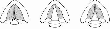
Figure
2.1 Vocal fold abduction and adduction during phonation. Axial view
from above the vocal folds. The leftmost figure shows closure of the vocal
folds along its length up to the two arytenoid cartilages. From [63].
Two effects of the DC flow offset are observed. First, the
degree of the DC offset could be correlated with other aspects of the glottal
waveform such as AC amplitude and opening and closing characteristics. The
influence of the DC offset in this case is schematized in Figure 2.2a. Secondly, the DC term could simply act as a strict
vertical offset so that the opening and closing characteristics of the waveform
are not changed. Figure
2.2b schematizes this process.
|
(a)
|
(b)
|
Figure 2.2 Effect
of the DC offset parameter on the glottal flow velocity waveform, DC = 0
(dashed line) and DC = 0.2 (solid line). (a) Increase in DC offset is
accompanied by a decrease in the AC amplitude, and (b) increase in DC offset
strictly vertically offsets the entire waveform. Pitch period is 0.01 s.
Empirical observations support both processes of Figure 2.2 in different cases. In one research study, Holmberg,
Hillman, and Perkell derive inverse-filtered waveforms for the vowel /a/ from
the oral airflow of male and female speakers at different loudness levels [27]. A DC offset was observed in
the inverse-filtered waveform, especially when the vowel was phonated at a soft
level. The effect of the DC offset mirrored what is schematized in Figure 2.2a. An increase in the DC flow was accompanied by a
decrease in the AC amplitude of the airflow. In addition, the data point to a
simultaneous increase in open quotient and rounding of the corners at the
opening and closing portions of the waveform.
At a constant production level, however, the varying sizes of
the glottal chink can be observed in the acoustics [27]. Empirical observations
closely mirror the simulated glottal waveforms in Figure 2.2b. This process would lend itself to the notion that
closure of the vocal folds maintains its abrupt nature even when a DC flow is
observed. The two mechanismsthe
AC waveform and the DC offsetare
distinct and almost decoupled since each is due to a different portion of the
vocal folds. Care must be taken to ascribe the AC waveform to the vibration of
the membranous portion of the vocal folds, while the DC offset is due to the
non-vibrating cartilaginous portion of the vocal folds. In the model and
implementation that follow, the schematic in Figure
2.2b is selected as the effect of DC flow on the glottal
volume velocity source.
Within a given speaker, the loudness level can significantly
modify the glottal waveform, potentially affecting the AC amplitude of the
noise source as well as open quotient and the abruptness of vocal fold opening
and closure [27]. These secondary phenomena
are not taken into account.
Inspired by the above-mentioned physiological observations, we
develop a model for the production of a vowel. The temporal characteristics of
the noise sourcemodulations
at the rate of the fundamental frequency and DC flowand
the observed broadband spectral characteristic will be taken into account. A block
diagram summarizes the model in Figure
2.3. The output waveform consists of a linear sum of both
a periodic and noise component. The periodic component is the output of the
linear vocal tract filter with a periodic glottal flow velocity source, while
the noise component is the output of the vocal tract filter with a modulated white
noise input.
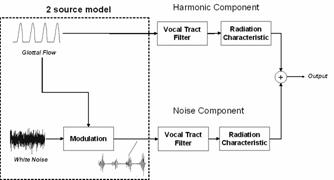
Figure
2.3 Vowel production model.
To put this flow diagram into
formal equations, it helps to view the signals of interest in the time domain (from
[63]). The periodic source, ,
arises from the periodic vibrations of the vocal folds and can be represented
by one period of the glottal flow velocity waveform, ,
convolved with a train of impulses, ,
with its period equal to the inverse of the fundamental frequency:
|
|
|
(2.1)
|
This volume velocity source is
input into a linear time-invariant filter representing the vocal tract, with
impulse response ,
which effectively filters and shapes the spectrum of the glottal source. The
output signal at the lips due to the periodic source, ,
is thus
|
|
|
(2.2)
|
In the model of the noise
component, air flows through the constrictions at the glottis and encounters obstructions
that generate turbulence, which aggregates into a noise source denoted by .
This noise source is effectively gated and modulated by the opening and closing
of the vocal folds, where the modulation function is represented by and is assumed multiplicative. The model
assumes that the modulated noise source, ,
is then input into the same vocal tract filter that operates on the periodic
glottal source. The output signal at the lips due to the noise source is :
|
|
|
(2.3)
|
Both and are volume velocity signals. The periodic
portion is due to the periodic puffs of air generated at the glottis, and the
noise portion is due to the acoustic realization of airflow turbulence at the
glottis.
The overall signal that a
standard condenser microphone measures manifests as acoustic pressure waves that
propagate through the ambient air. Since the pressure signal is measured by the
microphone at a certain distance from the lips, a transformation occurs from
the volume velocity signals and to the pressure signals due to the radiation
impedance in the atmosphere. Assumed to be a spherical acoustic source, the
volume velocity signals at the lips are passed through a filter representing
this radiation characteristic, which, in continuous time, is given by (a
far-field approximation valid for frequencies up to 4000 Hz) [73]:
|
|
|
(2.4)
|
where is the density of air, is the distance from the velocity source to a far-field
microphone, and is the speed of sound. We are usually
concerned with the magnitude of the radiation characteristic, ,
approximated by [73]
|
|
|
(2.5)
|
The magnitude of the radiation characteristic filter is
effectively linearly proportional to frequency and thus emphasizes energy at
higher frequencies. The discrete-time filter associated with is denoted by .
The output pressure signal in
the production model reflects the presence of the radiation characteristic. The
total speech pressure signal at the microphone, ,
is modeled as the linear addition of the periodic and noise components:
|
|
|
(2.6)
|
In this section, we describe a MATLAB implementation of the production
model in Figure 2.3 above to synthesize an aspirated vowel. The implementation
is inspired by elements of the Klatt synthesizer and includes a periodic voicing
source (Klatt’s AV parameter) and a stochastic aspiration noise source (Klatt’s
AH parameter) [36, 37].
The form chosen for the periodic source is a pulse shape by
Rosenberg used in the Klatt synthesizer as the KLGLOTT88 source [36, 37]. Rosenberg has documented the
effect of various glottal pulse shapes on listeners’ perception of natural
voice quality [67], and the main result is that
listeners are not significantly receptive to differences in fine time structure
of the source shape. A parametric polynomial fit to the shape of the periodic
source, the classic Rosenberg
pulse, was shown in that study to produce a natural quality when synthesizing
vocalic speech sounds. The simplicity of this function and the lack of need to
have detailed control over other glottal source parameters were factors in
choosing the Rosenberg model (see [9, 17, 18] for more complex forms).
The equation for the Rosenberg model, ,
of the glottal pulse in continuous time is
|
|
|
(2.7)
|
where is the open quotient (fraction between 0 to 1)
and is the fundamental period in Hz. The waveform
is sampled at sampling rate to yield the discretized waveform, ,
in Equation (2.1).
As mentioned above, the periodic
source is implemented as the derivative of the glottal flow velocity,
effectively taking into account the high-pass radiation characteristic. After
this radiation characteristic is folded in, the derivative of Equation (2.7) yields the effective excitation to the acoustic
filter of the vocal tract. The resulting glottal flow derivative, ,
is simply
|
|
|
(2.8)
|
After sampling this waveform at ,
the resulting signal is ,
an approximation to the derivative of the glottal airflow waveform.
The rationale behind keeping the volume velocity waveform in
the block diagram is due to an important assumption in the model that, before
vocal tract filtering, the noise source is modulated by the glottal airflow
waveform. This implementation differs from the approach of the Klatt
synthesizer, in which the aspiration noise is simply modulated by a square wave
with duty cycle equal to the open phase duration [36]. To emphasize our assumed
coupling between the periodic and aspiration noise source, the periodic
excitation is left undifferentiated in the production model of Figure 2.3. A sample glottal airflow waveform and corresponding
derivative are shown in Figure
2.4. Arrows indicate open and closed phase portions of
the waveform.
Figure 2.4 Glottal
airflow velocity waveform. Rosenberg
model (top) and its corresponding derivative waveform (bottom) representing the
effective periodic input as a pressure source. = 0.01 s, = 0.6, = 8000 Hz.
The waveforms are vertically offset for clarity.
The aspiration noise source consists of AC and DC
characteristics. The following sections clarify the implementation of these two
components.
AC Component
Synthesis assumes that the aspiration noise amplitude is
modulated by the area of the glottal opening, which is assumed to be related to
the glottal airflow velocity function, (Figure
2.4, top). Thus, concomitant with the volume velocity
source due to the periodic vocal fold vibrations is the volume velocity source
due to turbulent airflow at the glottis. Using the notation of Equation (2.3), the aspiration noise source is ,
where represents the aggregate contribution from all
glottal noise sources. We assume that is from a zero-mean white Gaussian
distribution and represents noise sources that occur at several locations
around the glottis. Delays between sources are not currently modeled. Figure 2.5 displays a synthesized example of the AC component of
the aspiration noise source. The glottal waveform, ,
modulates the white Gaussian noise source, .
The result is the AC component of the aspiration noise source, .

Figure 2.5 The AC component of the aspiration noise
source. Glottal waveform (top), white Gaussian noise signal (middle), and noise
signal modulated by the glottal waveform (bottom). = 0.01 s, = 0.6, = 8000 Hz. The waveforms are vertically offset
for clarity.
DC Flow
In the discussion on vocal fold mechanics in Section 2.1, it was concluded that, for constant sound level
production, the DC flow simply acts as a vertical offset to the AC waveform
with zero offset (recall the bottom signal in Figure
2.5). This is the source signal model implemented in the MATLAB
code and illustrated in Figure
2.6. Depending on the choice for the DC synthesis
parameter, the glottal waveform is generated and acts as the noise modulation
function. Figure 2.7 contrasts an unmodulated noise source with modulated
sources with two different DC offsets.
Figure 2.6 The DC component of the aspiration noise
source. The glottal flow velocity waveform with no DC flow (dashed line) and DC
flow of 0.2 (solid line). = 0.01 s, = 0.6, = 8000 Hz.
Figure 2.7 Generating the modulated aspiration noise
source. (a) Unmodulated white Gaussian noise, (b) noise signal modulated by
glottal waveform with no DC flow, and (c) noise signal modulated by glottal
waveform with a DC flow of 0.2. = 0.01 s, = 0.6, = 8000 Hz.
The vocal tract is modeled as a
cascade of three second-order filters or, as Klatt refers to them as, “digital
formant resonators” [36, 37]. Each of the three digital
resonators is in the form (z-domain):
|
|
|
(2.9)
|
where
and is the bandwidth of the formant, is the formant frequency, and is the sampling rate, all in Hz. Multiplication
of three of these transfer functions results in the overall transfer function
of the desired three-formant vocal tract configuration, with impulse response, .
Formant frequencies and bandwidths used in this study are tabulated in Table 2.1. Although higher formants could have been included,
it was decided to only draw from the Peterson and Barney data [62] and reduce complexity for the
current analysis.
|
Phonetic
Symbol
|
Synthesizer
Symbol
|
Male
|
Female
|
|
|
|
F1
|
F2
|
F3
|
F1
|
F2
|
F3
|
|
/i/
|
i
|
270
|
2290
|
3010
|
310
|
2790
|
3310
|
|
/e/
|
e
|
460
|
1890
|
2670
|
560
|
2320
|
2950
|
|
/æ/
|
ae
|
660
|
1720
|
2410
|
860
|
2050
|
2850
|
|
/a/
|
a
|
730
|
1090
|
2440
|
850
|
1220
|
2810
|
|
/o/
|
o
|
450
|
1050
|
2610
|
600
|
1200
|
2540
|
|
/u/
|
u
|
300
|
870
|
2240
|
370
|
950
|
2670
|
Table 2.1 Vowel formant frequencies, in Hz. Data from
[62] and [73].
Eliminating the need to explicitly indicate the density of air
or a distance in Equation (2.5), the digital filter representing the radiation
characteristic, ,
is often implemented as a first-difference filter, approximating its high-pass
characteristic and is (in the z-domain)
|
|
|
(2.10)
|
Synthesis equations have been developed above for the glottal
airflow waveform ,
the derivative of the glottal waveform ,
and the aspiration noise source prior to modulation due to the gating effect
of vocal fold oscillations. Formulae were also derived for the effect of
modulations and DC offsets on the aspiration noise source, as well as for the
acoustic filter properties of the vocal tract. Variables for the synthesizer
are set by nine synthesis parameters (see Appendix A for list with default values). It is noted that the
addition of perturbations such as frequency jitter and amplitude shimmer would
form a more complete synthesis system [21, 36, 37, 55, 56], especially when modeling
disordered speech [10, 40, 51]. The analysis and
modification sections in the following chapters do not include jitter and shimmer
parameters; however, their anticipated effects are investigated for future improvements
(Section 5.1).
For flexibility, the aspiration noise can either be modulated
or unmodulated by the glottal airflow waveform. Six vowels are chosen for
investigative purposes. The three formants to be used in the vocal tract resonators
of Equation (2.9) are selected by the vowel and the gender parameters,
as indicated in Table
2.1. Differences in oral and pharyngeal cavity lengths for
males and females correlate with different average formant frequencies [73]. The fundamental frequency
parameter, f0, is set for each glottal cycle, and the sampling rate and
duration of the vowel are set as desired.
The last three synthesis parameters
are DC, OQ, and HNR, which set important attributes of the source signals. DC
determines the DC offset on the glottal flow waveform as a fraction of the AC
amplitude. OQ indicates the open quotient during a glottal cycle, defined as the
ratio of the open-phase to closed-phase duration. Finally, the
harmonics-to-noise ratio (HNR) sets the ratio of the powers in the harmonic and
noise components computed on the signals after filtering by the vocal tract resonances
and the radiation characteristic. HNR is defined as
|
|
|
(2.11)
|
where is the harmonic component, is the noise component, and is the signal length. See Appendix A for a list of the vowel synthesizer’s parameters and
Appendix B for a graphical user interface created for developing
code and performing simulations with different test parameters.
The linear source-filter model detailed above, in which the
nonlinear modulation is folded into the noise source, is not the only way that
one may view the production of voiced speech. Notions of the involvement of
non-acoustic components contributing to spectral characteristics of the speech
pressure signal were introduced, for example, by Teager [77], further qualitatively
evaluated by Kaiser [33], and more recently
investigated experimentally by several research groups [3, 39, 49, 52, 71, 81]. The essence of these models
of aeroacoustics in speech production rests on the existence of concomitant
airflows of vortices in the vocal tract and pharyngeal region.
In one study, measurements of velocity and pressure in a simple
mechanical model of the vocal folds and vocal tract seem to indicate the
presence of such a non-acoustic component at the source of the mechanical
model. The non-acoustic source energy, following a transformation to acoustic
energy, is shown to contribute to the power spectrum of the output pressure
signal [3, 71]. Evidence thus points to the
possibility of aerodynamic influences contributing to the source and to formant
shaping [77]. Although aerodynamics and
other non-acoustic phenomena must be fully accounted for in a complete model of
speech production, implementation is computationally intensive and beyond the
scope of this study. The linear source-filter theory provides a flexible
paradigm that can be readily adapted for the current study.
After developing and
implementing the vowel synthesizer, it was desired to obtain a flavor for the
perceptual salience of different noise characteristics. For this purpose, this
section reviews some earlier work as well as our informal evaluation of the
perception of these synthesized vowels. In particular, the perceptual experiments
performed by Hermes [20] motivated the current preliminary investigation.
In his work, Hermes investigates the synthesis of a natural breathy voice quality
using an additive model with impulsive and stochastic sources. Hermes documents
the perceptual consequences of synthesizing the stochastic source with various
characteristics in both the time and frequency domain.
The next three
sections briefly investigate time- and frequency-domain characteristics of the
aspiration noise source and provides some informal observations of their effect
on human perception. Section 2.5.1 comments on differences in perception when the vowel
is synthesized either with an unmodulated or modulated noise source. Section 2.5.2 investigates the possible perceptual effects of
imposing different modulation functions on the aspiration noise source.
Finally, Section 2.5.3 introduces the importance of synchrony between the
modulated noise and the periodic excitation, drawing from one of Hermes’
experiments [20].
Hermes investigates
the fusion of periodic and noise components when synthesizing breathy vowels
and concludes that noise bursts must lie in phase with the glottal pulse
excitation for maximum “fusion” with the periodic sound component [20]. References are made to Bregman’s theory of
auditory scene analysis [5], in which two auditory objects may fuse
together only if they both contribute to the overall timbre of the sound. As a
consequence, if an unmodulated noise were used for aspiration source synthesis,
a percept of two streams may resultone
due to the periodic source and the other due to the unmodulated noise source.
Figure 2.8 displays two synthesized sources illustrating the temporal
differences between an unmodulated and modulated noise source. In this example,
the modulating function is taken to be the glottal airflow waveform, although
Hermes did not define a specific shape. Section 2.5.2 will present work on comparing the perception of different
modulation functions.
|
(a)
|
(b)
|
Figure 2.8 The
aspiration noise source. (a) Unmodulated white Gaussian noise and (b)
noise signal modulated by glottal waveform. Synthesis parameters: f0=
100 (pitch period = 0.01 s), fs =
8000, DC = 0.2, OQ = 0.6.
In Hermes’ work and in
our informal listening, after filtering by the vocal tract formants and
radiation characteristic, the vowel’s noisy part seems to perceptually
integrate better with the periodic component when modulated noise is used as
the aspiration noise source. These results indicate that modulation may be
important for the synthesis of a natural-sounding vowel but do not reveal how
best to select the modulation function.
Modulation of the
noise component in the time domain seems to be perceptually significant and
physiologically plausible, a view adopted by many researchers (e.g., [38]). Klatt, however, states that no evidence
supports the use of any specific modulation function, as long as a modulation
function exists [36-38]. It is desirable to further explore the
perception of different modulation functions on the aspiration noise source.
Four different
modulation patterns are chosen for study and illustrated in Figure 2.9. The functions are a rectangle, a sinusoid, and a glottal
airflow velocity waveform with and without a DC component. Vowels are
synthesized with the noise sources modulated by each function. Informal
listening indicates that the glottal airflow waveform provides for the most
natural synthesis, with a non-zero DC component slightly preferred to zero DC. Rigorous
listening tests, however, would need to be performed to statistically support
this conclusion.
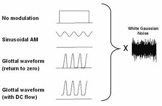
Figure
2.9 The
four modulation functions imposed on the aspiration noise source. Rectangle (no
modulation), sinusoidal amplitude modulation, the glottal waveform with no DC component,
and the glottal waveform with a DC component.
A speculation of
Hermes’ work is that, to be perceptually fused, the noise bursts at the source
lie in a certain phase with the concomitant periodic source [20]. Our work investigates the synchrony issue
and takes a step further to use a glottal waveform model (the Rosenberg pulse in Section 2.3.1) to represent the periodic source, unlikely Hermes’
impulsive excitation. Figure
2.10 illustrates how the sources would be synthesized when
the periodic excitation is in phase or out of phase with the aspiration noise
source. The in-phase case synthesizes the sources so that the noise maxima
occur near the location of peak air flow, imposed by the modulations of the periodic
source.
|
(a)
|
(b)
|
Figure
2.10 Perception
of source synchrony. (a) In-phase and (b) out-of-phase source waveforms. Synthesized
glottal waveform (dotted line), derivative of glottal waveform (top solid
line), and aspiration noise source (bottom solid line). Synthesis parameters:
Noise type = modulated, Vowel = a, f0=
100, Gender = m, fs = 8000, Duration = 1,
DC = 0.1, OQ = 0.4, HNR = 10. The waveforms are vertically offset for clarity.
The waveforms are then
the periodic- and noise-source inputs to the vowel synthesizer of Section 2.3. Note that the pitch is held constant to allow a
constant time offset to uniformly shift the entire noise signal so the noise
maxima occur in the same phase within each cycle. Our preliminary perception of
the two synthesized vowels agree with Hermes’ conclusion that there is less
roughness in the output signal when the signals in Figure 2.10a are sources. Hermes would say that the listener
would hear the out-of-phase sources in Figure
2.10b as two perceptual auditory streams or objects. Indeed,
the vowel synthesized from these sources sounds less natural and likely to
arise from two distinct sources.
In this section, we
first described the essential physiological mechanisms of speech production and
developed a linear source-filter model to describe the effects of these mechanisms.
A vowel synthesizer was implemented in MATLAB [47], and we detailed each stage of processing
with equations in Section 2.3. The entire synthesis system resembles the Klatt
synthesizer [36, 37], but with a key difference when
implementing the aspiration noise source. Instead of selecting an arbitrary
modulation function imposed on the noise source, the periodic volume velocity
waveform is chosen as the specific modulation function.
Alternative speech
models were briefly mentioned in Section 2.4, introducing the importance of aerodynamic
parameters. Due to its complexity and its computational load, these models are
outside the scope of the current study. Finally, we reviewed earlier work by
Hermes [20] and Klatt [38] and made our own preliminary observations
on the perception of the natural quality of synthesized vowels with a modulated
aspiration noise source. Specifically, we addressed the perceptual salience of
noise modulations, the specific modulation function, and the synchrony of the
periodic and noise components.
Chapter 2 provides us with a framework within which we can test
our analysis and modification algorithms. With knowledge of the input source
signals in the synthesizer, we can derive performance measures to assess the
accuracy of an analysis tool that extracts the periodic and noise components in
speech. Building this harmonic/noise separation algorithm is the subject of
Chapter 3.
Chapter 3
In Chapter 2, we developed an additive noise model to represent
the speech signal during phonation as the sum of a periodic or harmonic
component and an aspiration noise component. We then developed a vowel synthesizer
based on this model that provides access to the waveforms at each stage of synthesis.
In Chapter 3, we now develop a tool to analyze the harmonic and
noise components of both synthesized and real vowels.
Section 3.1 begins with an overview of current harmonic/noise
analysis algorithms and their limitations. We choose one of these algorithms,
the pitch-scaled harmonic filter [31], for further analysis and discuss
its MATLAB implementation in Section 3.2. Sections 3.3 and 3.4 are devoted to examples of harmonic/noise component
analysis on synthesized and real vowels.
All separation algorithms seek to first estimate the periodic
portion of a signal, followed by a temporal or spectral subtraction step. Although
some speech processing algorithms assume that the noise and periodic components
of voiced speech spectrally overlap, they ultimately simplify the analysis by
assuming that the noise component lies solely in a high frequency region [43, 75]. Recently, a number of
decomposition techniques have been introduced that show improved accuracy at
estimating the harmonic and noise components with accurate spectral and
temporal resolution [7, 31, 80]. The resulting signals can
then be analyzed for interesting traits in the frequency and time domains.
Three harmonic/noise separation algorithms are described in this
section. Section 3.1.1 describes state-of-the-art algorithms for separating
the harmonic and noise components of a signal. Section 3.1.2 presents limitations of these algorithms and
motivates the selection of one of them for continued analysis and use in our
study.
Yegnanarayana et al. [7, 8, 80] propose a decomposition
method that incorporates inverse filtering and a cepstral lifter (analogous to
a spectral comb filter) to initially separate the harmonic and noise
components. The authors take the stance that each DFT coefficient contains a
contribution from both a periodic component and a noise component. First,
inverse filtering is accomplished by an all-zero whitening filter whose
coefficients are calculated using linear prediction. An argument for this first
step is that, since both the periodic and noise components are generated at the
source level, decomposition should be performed on the excitation signal, or residual
signal after inverse filtering. Second, the authors convert the residual
excitation signal to the cepstral domain and lifter out the periodic excitation
energy in quefrency. This provides initial estimates for the periodic and aperiodic
excitation components. Since the resulting aperiodic spectrum contains gaps at
harmonic frequencies, an iterative algorithm is developed to converge to an
optimized estimate of the aperiodic excitation. Time-domain subtraction from
the original residual signal results in the estimate of the periodic component
of the source excitation. Each source component is then filtered by an all-pole
filter whose coefficients come from the whitening step.
A second decomposition method, by Jackson and Shadle [29-31], provides a purely spectral
technique that places a comb filter on the output pressure signal (no inverse
filtering) to arrive at the harmonic component of the signal. The approach uses
an analysis window duration equal to a small integer number of pitch periods
and relies on the property that harmonics of the fundamental frequency fall at
specific frequency bins of the discrete short-time Fourier transform. Thus, the
pitch at each analysis time instant must be estimated prior to comb filtering. Since
the comb filter only passes frequencies in harmonics of the fundamental
frequency, the algorithm is referred to as the pitch-scaled harmonic filter
(PSHF). To fill in gaps that occur in the residual noise spectrum (as also with
the algorithm by Yegnanarayana et al.), spectral power interpolation is
performed prior to the inverse DFT. Specifics
of the algorithm’s implementation are presented in Section 3.2.
Prior to the PSHF, Serra and Smith [70] developed an alternative spectral-based
decomposition algorithm. The authors also perform spectral subtraction to
separate the periodic and noise components and use the inverse DFT to arrive at
the desired extracted signals. An important difference from the PSHF, though, is
that Serra and Smith do not restrict the deterministic part of the signal to contain
harmonically-related frequency components. This probably results from the
authors’ interest in analyzing non-harmonic music signals, as well as speech. Instead
of filtering each analysis frame whose length depends on the local pitch (as was
the case in the PSHF algorithm), Serra and Smith employ a peak-picking
algorithm in the short-time spectra to identify energy contributions from the
deterministic part of the signal. The algorithm then follows that of the PSHF
method, similarly including a interpolation stage to fill in spectral gaps.
A summary of the major features of each of the three algorithms
described above is presented in Table
3.1.
|
Researchers
|
Analysis
domain
|
Subtraction
domain
|
Harmonic
constraint?
|
|
Yegnanarayana
et al. [7, 8, 80]
|
CD/FD
|
TD
|
Yes
|
|
Serra
and Smith [70]
|
FD
|
FD
|
No
|
|
Jackson
and Shadle [29-31]
|
FD
|
FD
|
Yes
|
Table 3.1 Comparison of harmonic/noise
decomposition algorithms. TD = time domain, FD = frequency domain, CD =
cepstral domain.
The performance of an iterative algorithm like that by
Yegnanarayana et al. [7, 8, 80] is pre-disposed to robustness
issues. Both the use of a linear predictive analysis front-end and the inclusion
of an iterative algorithm have been discounted as being ineffective by Jackson
and Shadle [31]. They show the iterative
algorithm to ultimately converge to the original residual excitation signal
that includes both periodic and aperiodic factors. In addition, whitening by
inverse filtering is not viewed as helping improve spectral analysis of the
signals, as linear prediction analysis has its own assumptions and limitations.
Regarding the Serra and Smith algorithm [70], although harmonicity is not
assumed, stochastic variations in the spectrum could lead the system to
incorrectly assign a particular DFT bin as deterministic. As a result, the
harmonic assumption will be taken in the current study because speech signals
tend to behave under this constraint during voicing.
We chose the PSHF since Jackson and Shadle claim that the
algorithm can preserve the temporal modulation characteristics of the noise
component and approximately isolate the
noise component from a voiced fricative signal [29, 31]. Some leakage of harmonicity can be present
in the extracted noise component [50], and the presence of shimmer and
jitter provides difficulty (see Section 5.1 for a discussion). For shimmer and jitter ranges observed in normal speakers, however,
Jackson and
Shadle claim that the PSHF can be used as an effective analysis tool [31]. Our implementation of the
PSHF and example analyses using the algorithm are described in the following
sections.
The pitch-scaled harmonic filter (PSHF) technique was implemented
in MATLAB [47] to operate on an input speech
signal, .
Short-time analysis is performed on a windowed portion of to result in two signals, a harmonic and a
noise component. Overlap-add synthesis is then used to merge together all the
short-time segments (see [63] for a discussion on the OLA analysis/synthesis
framework). Details of the PSHF can be found in [31], but we present the critical components
below.
Every 10 ms, the local pitch period, ,
is estimated. Pitch estimation is accomplished using the speech signal
processing tool Praat [4]. The Praat algorithm arrives
at a periodicity measure by a forward cross-correlation analysis [4]. The PSHF imposes an analysis
window of length ,
which will be shown to be time-dependent. The window employed is the Hanning
window, :
|
|
|
(3.1)
|
Using the classic
overlap-add analysis method, each short-time segment, ,
is thus
|
|
|
(3.2)
|
where is the frame number and is the frame advance. The frame index, ,
will be dropped for the moment for clarity and reintroduced during overlap-add
synthesis.
Estimation of the periodic component assumes harmonicity and relies
on the property that if is chosen appropriately for each time instant,
the harmonics will fall at specific frequency bins of an -point discrete short-time Fourier transform, .
See Appendix C for an example analysis on a vowel signal
demonstrating this property.
The discrete spectrum of the
harmonic component of a frame, ,
is thus given by:
|
|
|
(3.3)
|
where is the DFT index and is the set .
After obtaining an estimate for the harmonic component, spectral
subtraction is subsequently performed to obtain the spectrum of the noise
component estimate, :
|
|
|
(3.4)
|
where is the -point DFT of the rectangular-windowed single,
.
Note that zeroes exist in the discrete spectrum of at every th bin. Assuming that the envelope of the
power spectrum of the noise is smooth, additional processing interpolates power
estimates from neighboring bins to fill in the zeroed frequency regions. A
revised harmonic estimate is then obtained by taking into account the interpolated
noise power present in the harmonically-labeled bins.
The revised estimates of the harmonic
component, ,
and noise component, ,
are (from [31]):
|
|
|
(3.5)
|
|
|
|
(3.6)
|
where
The time-domain signals of the harmonic and noise
components in each frame are obtained by performing an -point inverse DFT, yielding and ,
respectively.
We can reconstruct the entire signals from the short-time
segments by re-introducing the time dependence (frame index ) and using overlap-add synthesis [63]:
|
|
|
(3.7)
|
|
|
|
(3.8)
|
where is the number of segments in each signal. Note
that the normalization factor in the denominator is due to window weighting on
each short-time segment. The sum of overlapping Hanning windows will not be
equal to one, and as a consequence, the overlap-add method divides out the
effect of the window sum.
This section analyzes a synthesized vowel
with a steady pitch. It is instructive to first analyze synthesized vowels
since the periodic and noise components are known inputs in the synthesis
framework described in Chapter 2. After estimating these components from the overall
pressure signal (assuming no knowledge of the input sources), direct comparisons
can be made to assess confidence in the decomposition technique. Other example
vowels are then analyzed in Section 3.4.
Two assessment measures can be devised for
the two outputs of harmonic/noise decomposition. One measure deals with the
frequency-domain characteristics and overall power levels. The other, more
qualitative, assessment compares the time-domain characteristics of the input
and output waveforms. The synthesis framework gives us access to the building
blocks of the vowel. The main synthesis parameter that will be varied for
performance assessment of decomposition is the harmonics-to-noise ratio (HNR). The
HNR serves as an indication of the relative level contributions of the harmonic
component and the noise component. HNR is defined as
|
|
|
(3.9)
|
where is the estimated harmonic component, is the estimated noise component, and is the signal length. Ideally, the HNR value
set during synthesis will be equal to the HNR calculated on the extracted
components. This allows one to observe any consistent overestimation or
underestimation of the power in a specific component.
Table
3.2 displays the results of the analysis of one
synthesized vowel. Synthesis parameters are indicated in the caption, with the
aspiration noise source being unmodulated. It is noted that due to the
stochastic nature of the original signal, it is unreasonable to expect an input
random signal to be perfectly reconstructed at the output. The overall
statistics, however, are assumed to be unchanged. Table 3.3 calculates performance measures for another
synthesized with the same synthesis parameters, except the noise source type is
modulated.
|
HNRinput
(dB)
|
HNRoutput
(dB)
|
ΔHNR
(dB)
|
Periodicinput
(dB re
1 Volt)
|
Periodicoutput
(dB re
1 Volt)
|
Noiseinput
(dB re
1 Volt)
|
Noiseoutput
(dB re
1 Volt)
|
|
-20.0
|
-5.1
|
+14.9
|
-42.5
|
-28.8
|
-22.5
|
-23.6
|
|
-15.0
|
-5.0
|
+10.0
|
-38.4
|
-29.5
|
-23.4
|
-24.5
|
|
-10.0
|
-2.9
|
+7.1
|
-34.4
|
-28.6
|
-24.4
|
-25.7
|
|
-5.0
|
-4.6
|
+0.4
|
-29.3
|
-29.1
|
-24.3
|
-24.5
|
|
0.0
|
+2.5
|
+2.5
|
-25.8
|
-25.0
|
-25.8
|
-27.6
|
|
+5.0
|
+6.7
|
+1.7
|
-22.9
|
-22.8
|
-27.9
|
-29.5
|
|
+10.0
|
+11.2
|
+1.2
|
-21.5
|
-21.6
|
-31.5
|
-32.8
|
|
+15.0
|
+15.8
|
+0.8
|
-20.9
|
-20.9
|
-35.8
|
-36.7
|
|
+20.0
|
+19.7
|
-0.3
|
-20.3
|
-20.4
|
-40.3
|
-40.1
|
|
+25.0
|
+22.7
|
-2.3
|
-19.9
|
-20.0
|
-44.9
|
-42.7
|
|
+30.0
|
+23.9
|
-6.1
|
-19.7
|
-19.8
|
-49.7
|
-43.7
|
Table 3.2 HNR
measures for harmonic/noise analysis of synthesized vowel with unmodulated
aspiration noise source. Noise type = unmodulated, vowel = a, f0 =
100, Gender = m, fs = 8000, Duration = 1, DC = 0.1, OQ = 0.6. Parameter
is HNR.
|
HNRinput
(dB)
|
HNRoutput
(dB)
|
ΔHNR
(dB)
|
Periodicinput
(dB re
1 Volt)
|
Periodicoutput
(dB re
1 Volt)
|
Noiseinput
(dB re
1 Volt)
|
Noiseoutput
(dB re
1 Volt)
|
|
-20.0
|
-3.5
|
+16.5
|
-45.0
|
-30.5
|
-25.0
|
-27.0
|
|
-15.0
|
-4.7
|
+10.3
|
-38.9
|
-30.1
|
-23.9
|
-25.4
|
|
-10.0
|
-4.9
|
+5.1
|
-35.0
|
-31.3
|
-25.0
|
-26.3
|
|
-5.0
|
-3.9
|
+1.1
|
-30.5
|
-30.0
|
-25.5
|
-26.1
|
|
0.0
|
+2.4
|
+2.4
|
-26.2
|
-25.8
|
-26.2
|
-28.2
|
|
+5.0
|
+6.6
|
+1.6
|
-24.1
|
-24.1
|
-29.1
|
-30.7
|
|
+10.0
|
+11.3
|
+1.3
|
-21.5
|
-21.4
|
-31.5
|
-32.7
|
|
+15.0
|
+16.2
|
+1.2
|
-20.9
|
-20.9
|
-35.9
|
-37.1
|
|
+20.0
|
+19.8
|
-0.2
|
-20.1
|
-20.2
|
-40.1
|
-40.0
|
|
+25.0
|
+22.6
|
-2.4
|
-19.8
|
-19.9
|
-44.8
|
-42.4
|
|
+30.0
|
+23.9
|
-6.1
|
-19.7
|
-19.8
|
-49.7
|
-43.6
|
Table 3.3 HNR
measures for harmonic/noise analysis of synthesized vowel with modulated
aspiration noise source. Noise type = modulated, vowel = a, f0 = 100, Gender = m, fs
= 8000, Duration = 1, DC = 0.1, OQ = 0.6. Parameter is HNR.
A plot of output HNR versus input HNR is
shown in Figure
3.1, in which the optimal function is a straight line
with unit slope. For HNRs between -5 and +20 dB, the relative power levels of
the estimated harmonic and noise components lies within about 3 dB of the known
input component levels. As HNRs decrease below -5 dB, the output HNR measure
stays approximately constant, indicating a ceiling of performance. In these
cases, zero regions can be seen in the waveform of the extracted harmonic
component. These gaps are partly due to the Praat pitch tracker not being able
to calculate a pitch estimate during specific time frames, understandable since
the stochastic signal begins to swamp out the harmonic part. Most of the output
noise component thus is equal to the input, which contains both harmonic and
stochastic elements.
Figure 3.1 Output
HNR vs. input HNR. Synthesized noise source is either unmodulated (circles) or
modulated (triangles). Dashed line indicates ideal performance with HNR equal
at input and output.
Since we are dealing with stochastic
signals, we can only estimate their power spectra and try to minimize biases
(deviations from the true mean) and variances (deviations from the true
variance). Bartlett’s procedure [60], a method for
averaging periodograms, is used to estimate the power spectra of the above
speech-like signals. The periodogram, ,
for a length- short-time segment, ,
windowed with a unit-height rectangle, is proportional to the squared magnitude
of the -point DFT with index [60]:
|
|
|
(3.10)
|
The periodogram itself is a biased estimate
of the true power spectrum of noise, with the expected value approaching zero
as more sample points are included in the window. For a given data length ,
however, increasing the number of samples per window results in decreasing the
number of windows available for averaging. This is a tradeoff, since increasing
the number of averaged periodograms reduces the estimate’s variance. The
parameters of Bartlett’s
procedure are (the entire signal length), (the window length), and (the number of samples to advance for each
successive window). The number of frames, ,
to be averaged falls out of the following equation:
|
|
|
(3.11)
|
where the function finds the largest integer smaller
than the argument. In the current analysis, a 50% window overlap was chosen, so
that .
The assumption of frame independence is not strictly maintained, but the
variance of the averaged periodogram has been shown to decrease nevertheless
with half-window overlapping [60]. With as the index for each periodogram from Equation
(3.10), the averaged periodogram is equal to
|
|
|
(3.12)
|
In subsequent plots, the individual
periodograms are calculated from short-time segments of length 50 ms. For a
1-second vowel sampled at 8000 Hz, the number of frames averaged, ,
is 38. Figure
3.2 displays for input and output signals from the PSHF of a
synthesized vowel with a modulated noise source. Figure 3.2c shows some harmonic leakage in the periodogram of
the noise component, especially in the 15002500
Hz frequency region. This leakage is due to small inaccuracies in the estimate
of the amplitudes at the harmonic frequencies in Figure 3.2b.
Figure 3.2 Averaged
periodograms of (a) synthesized vowel, (b) harmonic estimate, and (c) noise
estimate. In (b) and (c), superimposed are DFT magnitudes of the synthesized
harmonic and noise inputs, respectively. Synthesis parameters: Noise type =
modulated, Vowel = a, f0 = 100, Gender = m, fs = 8000,
Duration = 1, DC = 0.1, OQ = 0.6, HNR = 10.
In addition to desiring similar spectral
characteristics at the input and output, temporal features of the input signals
should be appropriately reconstructed in the extracted components. In the vowel
synthesizer, the noise source was modulated by the glottal flow velocity
function (the Rosenberg model in Figure
2.4), and so to view the modulations in the separated
noise component, sample waveforms from the PSHF output are displayed in Figure 3.3 and Figure
3.4.
Figure 3.3 Approximate
reconstruction of the harmonic component from the synthesized steady-pitch
vowel. Wideband spectrograms of (a) synthesized and (b) separated harmonic components,
and waveforms of (c) synthesized and (d) separated harmonic components.
Waveforms are shown on an expanded time scale. Synthesis parameters: Noise type
= modulated, Vowel = a, f0 = 100, Gender = m, fs = 8000,
Duration = 1, DC = 0.1, OQ = 0.6, HNR = 10.
The output harmonic estimate (Figure 3.3d) lines up in time with the known harmonic signal
input into the synthesizer (Figure
3.3c). This verifies the phase of the output. Wideband
spectrograms are computed for the synthesized component and estimate in Figure 3.3a and b, respectively. These, and subsequent,
spectrograms are computed with 4-ms Hanning analysis windows, half-window
overlap, and a 40-dB dynamic range. The variable-length analysis windowing
technique in the PSHF results in frequency bin estimates within 12
dB of the actual energy in the bin.
Of interest, also, is whether the envelope
energy fluctuations of the input white noise source are still present in the
extracted noise component at similar time locations. Figure 3.4 displays evidence that the envelope of the output
noise estimate contains local maxima and minima that occur at similar times to the
envelope of the input noise component.
Figure 3.4 Approximate
reconstruction of the modulated noise component from the synthesized
steady-pitch vowel. Wideband spectrograms of (a) synthesized and (b) separated noise
components, and waveforms of (c) synthesized and (d) separated noise
components. Waveforms are shown on an expanded time scale. Synthesis
parameters: Noise type = modulated, Vowel = a, f0 = 100, Gender = m,
fs = 8000, Duration = 1, DC = 0.1, OQ = 0.6, HNR = 10.
A time-domain pattern can be observed in the
spectrogram of the estimated noise component in Figure 3.4b, reflecting approximate fluctuations of the
synthesized aspiration noise in Figure
3.4a. Focusing on an expanded time scale of 100 ms, we
can make qualitative remarks on synchrony between modulations in the input and
output noise waveforms. The noise modulation pattern in the synthesized
waveform (Figure 3.4c) is evident at similar time instants in the noise
output of the PSHF algorithm (Figure
3.4d). Due to the stochastic nature of the signal and
estimation errors, though, exact reconstruction is not possible and thus noise
amplitudes are not identical at input and output.
To explore whether the modulations in the
noise output are not merely coincidental artifacts of the decomposition
algorithm, a synthesized vowel with unmodulated noise was input into the PSHF
analysis algorithm. Figure
3.5 displays wideband spectrograms of the input and
output noise components. As expected, regular temporal patterns are not
observable in the spectrogram of the synthesized, unmodulated aspiration noise in
Figure 3.5a. A closer look at the time structure reveals
envelope fluctuations of less regular modulation than the modulated noise
example in Figure 3.4, reflecting inherent stochastic fluctuations.
Figure 3.5. Approximate
reconstruction of the unmodulated noise component from the synthesized
steady-pitch vowel. Wideband spectrograms of (a) synthesized and (b) separated
noise components, and waveforms of (c) synthesized and (d) separated noise
components. Waveforms are shown on an expanded time scale. Synthesis
parameters: Noise type = unmodulated, Vowel = a, f0 = 100, Gender =
m, fs = 8000, Duration = 1, DC = 0.1, OQ = 0.6, HNR = 10.
Another important issue is whether the
modulations in the noise estimate are at the correct phase relationship with
the harmonic estimate; that is, the locations of noise source maxima should be present
during the open phase of the glottal volume velocity waveform. To better
observe these modulations in the noise source of the synthesized vowel, the output
noise estimate is inverse filtered to remove the effect of the vocal tract
filter. This operation utilizes a short-time whitening filter.
To whiten the spectrum, a Hanning window is
applied to a 20-ms analysis frame. Subsequent analysis frames overlap by half
the length of the window. Whitening is accomplished in each windowed segment by
the following algorithm: (1) estimating an all-pole model representing the
vocal tract filter spectral characteristics using linear prediction; (2)
inverse-filtering the short-time segment by a finite impulse response filter
whose tap weights are equal to the corresponding coefficients in the estimated
all-pole model; and (3) synthesis of the resulting signal through an
overlap-and-add process. Following the whitening operation, we can observe
modulations in the estimate of the noise source along with any synchrony with
the periodic component. A more detailed explanation of the whitening algorithm is
in Section 4.5.3.
Figure
3.6 displays the output of the whitening process (solid
line), representing an estimate of the aspiration noise source. Superimposed (dotted
line) is the known modulation functionthe
synthesized glottal airflow velocity waveformimposed
on the white Gaussian noise source. The desired temporal features are approximately
maintained. Maxima in the envelope of the estimated noise source occur during
the open phase of the glottal period, the location of the maxima of the
modulation function.
Figure 3.6 Temporal modulation structure approximately
preserved by PSHF algorithm. Whitened noise component estimate (solid line) and
synthesized glottal waveform (dashed line). Synthesis parameters: Noise type =
modulated, Vowel = a, f0 = 100, Gender = m, fs = 8000, Duration = 1,
DC = 0.1, OQ = 0.6, HNR = 10.
In their work with the PSHF separation
algorithm, Jackson and Shadle analyzed the noise components generated during
the production of voiced fricatives [29]. Complementing their
work, we analyze a different class of speech sounds, namely vowels that have a
noise component generated at the source. In Section 3.4.1, example harmonic/noise component analysis is
performed on a synthesized vowel with a time-varying pitch contour. Next,
Section 3.4.2 applies the PSHF algorithm on real vowels, one from a
normal speaker and another from a database of pathological speakers.
To better match the quality of a real vowel, we analyzed a
synthesized vowel whose pitch linearly increased from 100 to 140 Hz over a
one-second duration. The added pitch complexity tests the time resolution
capability of the PSHF algorithm, its ability to track changes in the
fundamental frequency of a waveform. Recall that the PSHF utilizes an analysis
window of four times the local pitch period, indicating a tradeoff between time
and frequency resolution due to the relatively long window length. Figure 3.7 displays the wideband spectrogram, pressure waveform,
and pitch contour of the first 0.5 seconds of the synthesized vowel.
Figure 3.7 Synthesized vowel /a/ with time-varying
pitch. (a) Wideband spectrogram, (b) pressure waveform, and (c) pitch contour. Synthesis
parameters: Noise type = modulated, Vowel = a, f0 = 100140,
Gender = m, fs = 8000, Duration = 1, DC = 0.1, OQ = 0.6, HNR = 10.
Figure 3.8 displays spectrograms and pressure waveforms of the
harmonic and noise estimates. As desired, the spectrograms indicate that the
harmonic estimate acquires most of the harmonic energy from the input signal (Figure 3.8a and c) and that the noise estimate is stochastic
with some patterns in the time domain (Figure
3.8b and d). A critical result lies in the
inverse-filtered version of the noise component estimate (Figure 3.8e). Knowing that the aspiration noise source was
modulated by an envelope function related to the glottal airflow, this airflow
waveform (normalized) is purposely superimposed on the inverse-filtered noise
waveform. As expected, the higher noise amplitudes are concentrated in the open
phase of the glottal airflow waveform.
Figure 3.8 Temporal
characteristics of harmonic/noise analysis on synthesized vowel with
time-varying pitch. Wideband spectrograms of separated (a) harmonic and (b)
noise components with pressure waveforms of (c) separated harmonic component,
(d) separated noise component, and (e) whitened noise component with synthesized
glottal waveform superimposed (dotted line).
3.4.2
Real Vowels
Up until now, the PSHF algorithm was tested on synthesized
vowels, where the output separated components could be compared with their
known synthesized counterparts. In this section, two real utterances are
analyzed, one from a normal speaker and another from a speaker with a diagnosed
vocal pathology.
Normal Speaker
The recording analyzed is of a non-pathological, male speaker.
The speaker utters the syllable /pæ/, in which the vowel yields a slightly breathy
percept. Figure 3.9 displays a wideband spectrogram and pressure waveform
of the utterance. Note that the first 0.75 seconds includes the noise bursts
due to the plosive release.
Figure 3.10 displays the outputs of the harmonic/noise analysis
by the PSHF technique. The separated noise component is notably weaker than the
harmonic component, supporting the perception that the breathiness quality is
not strong. Again, of note is the presence of modulation patterns in the
separated noise component. As was done in the analysis of the synthesized
vowels, an inverse-filtered version of the noise component is displayed to
estimate the source of the separated noise (Figure
3.10e). Dashed lines superimposed on the pressure
waveforms are placed at selected instants of assumed glottal closure. See
Appendix D for an explanation of how glottal closure instants
are derived from a speech waveform.
The amplitude maxima of the whitened noise waveform occur at
these instants; this is in extension to the time instants of noise source peaks
in the vowel production model of Figure
2.3, which assumed that noise maxima occurred during the
open phase of the glottal cycle. The results of this analysis indicate an
additional pattern. The modulation function on the estimate of the noise source
is observed to peak at instants of assumed glottal closure, as opposed to at the
peak of the open phase. This result extends our vowel production model and the
noise source structure in the Klatt synthesizer [36, 37], but consistent with
conclusions on source synchrony in [66].
These observations of synchrony between noise bursts and
assumed glottal closure are based on selected regions. For normal speaker
waveforms, we have observed other modulation patterns that are consistent with
the open-phase noise bursts in our vowel production model, as well as patterns
that are less distinctive in the estimated noise source waveform.
Figure 3.9 Utterance
by normal speaker, /pæ/. (a) Wideband spectrogram and (b) pressure waveform.
Figure 3.10 Temporal characteristics of harmonic/noise
analysis on /pæ/, uttered by normal speaker. Wideband spectrograms of separated
(a) harmonic and (b) noise components with pressure waveforms of (c) separated
harmonic component, (d) separated noise component, and (e) whitened noise
component. Dashed lines indicate sample instants of assumed glottal closure.
The plosive burst is vertically clipped in (d) to zoom in on the noise
modulations in the vocalic region.
Speaker with Vocal Pathology
We accessed a database of recordings from patients with
disordered voice characteristics [1] since aspiration noise in the
speech signal has been shown to correlate with certain vocal fold pathologies [23, 25, 26, 28, 40]. Armed with a tool to analyze
the harmonic and stochastic components of an acoustic pressure waveform, we can
now perform spectral and temporal analysis on the recordings of vowels produced
by pathological speakers.
One such recording was selected of a male patient with a
laryngeal assessment that indicated hyperfunction, anterior-posterior
squeezing, and ventricular compression [1]. These descriptors together
mean that the patient unconsciously seems to constrict the structures embodying
the laryngeal region, forcing him to “hyperfunction” or compensate by supplying
an increased air supply. This patient’s case is of particular interest due to
the diagnosis of a cyst on his vocal folds [1]. Due to common etiologies of
cysts, it is possible that the cyst is positioned on the medial edge of the
vocal folds as a scarring reaction to vocal fold trauma. The cyst could obstruct
the air supply from the lungs and act as a source of air turbulence. This additional
noise source would augment aspiration noise sources that are generated in the
normal case. Analysis of this patient’s noise source may, thus, lead to
acoustic markers of the cyst’s presence.
Averaged periodograms were computed over approximately one
second of phonation. The original spectrum, along with the spectra of the
extracted harmonic and noise components via the decomposition algorithm, is
plotted in Figure
3.11. Wideband spectrogram and pressure waveforms are
displayed in Figure 3.12. Immediate observations of the separated components yield
promising results, but spectral leakage exists. In the spectrum of the harmonic
component, the bulk of the energy is harmonic and exists below about 2000 Hz. Above
this frequency, however, noise-like energy exists is observed. Similarly, in
the noise spectrum, a small degree of harmonic energy is observed below 1500
Hz. These spectral leakages are possibly due to errors in pitch estimation and,
most probably, to high values of jitter and shimmer in the original speech
signal. The PSHF algorithm breaks down not only at high aspiration noise
levels, but also in the face of high jitter and shimmer values. Improving PSHF
performance on disordered voices having these perturbations is mentioned as an
issue deserving future analysis (Section 5.1).
Figure 3.11 Harmonic/noise
analysis speaker with vocal pathology. Periodograms of (a) synthesized vowel, (b)
harmonic estimate, and (c) noise estimate.
Analysis proceeds in the time domain as was done previously. Figure 3.13 displays sampled sections of the signals output from
the decomposition algorithm and an estimate of the source of the noise
component. Local peaks in noise amplitude are observed in the noise source
estimate. Furthermore, although some of these peaks coincide with the assumed
open phase of the glottis (vertical dashed line), other noise peaks occur at
times that coincide with the glottal pulse instants (vertical dotted line). Thus,
we see modulation phenomena similar to what was seen above in the normal
utterance and data that reflect our vowel production model. Fortunately,
although our model assumes only modulations with maximum noise amplitude during
the open phase, the decomposition algorithm makes no assumptions regarding
temporal characteristics of the extracted harmonic and noise estimates.
The aerodynamics interactions at the glottis act as an
additional source of noise in the airway, and this was alluded to above owing
to the presence of vocal fold cysts. Though these noise modulations have been
previously documented in analyses of pathological voices [28], the authors did not inverse-filter
the noise component to observe the characteristics of the source waveforms,
which we have shown to better illustrate the modulation function.
Figure
3.12 Sustained vowel /a/ uttered by speaker
with vocal pathology. (a) Wideband spectrogram and (b) pressure waveform.
Figure 3.13 Temporal characteristics of harmonic/noise
analysis on /a/ uttered by pathological speaker. Wideband spectrograms of
separated (a) harmonic and (b) noise components with pressure waveforms of (c)
separated harmonic component, (d) separated noise component, and (e) whitened
noise component. Left dotted line indicates sample instant of assumed glottal
closure. Right dashed line indicates sample instant of assumed peak in open
phase of glottal cycle.
Following the development of a modeling and synthesis framework
in Chapter 2, Chapter 3 dealt with the issue of separating the two additive
components in the modelharmonic
and noise. A review of three analysis techniques was presented, followed by
limitations of these techniques. Based on its published performance and ease of
implementation, the pitch-scaled harmonic filter (PSHF) algorithm was selected
for further analysis. The algorithm is developed in work by Jackson and Shadle
and documented in [29-31]. In Section 3.3, we submitted their algorithm to our own testing
using a vowel synthesized, in which all the input source waveforms are known.
Finally, Section 3.4 presented analysis of more natural vowels, including
one synthesized vowel and two human-produced vowels. One human-produced vowel
was from a normal speaker, and the other was from a speaker with a vocal
pathology.
Modulations in the noise source waveform and their synchrony
with the periodic source were shown to be important for natural-sounding vowel
synthesis in Section 2.5, and these modulations were approximately preserved
in the output of the PSHF algorithm. Although leakage of noise into the harmonic
component estimate was observed, we attribute the deviations to estimation
error and excessive levels of jitter and shimmer, a subject for further work (Section
5.1).
From our analysis of real vowels, we speculate that two types
of temporal modulations are present in the inverse-filtered version of the
separated aspiration noise component. Local peaks in noise amplitude seemed to coincide
with (a) the open phase of the glottal cycle and (b) time instants of glottal closure.
Thus, we see modulation phenomena that add to the modulation properties in our
vowel production model in Figure
2.5. Although the model assumes only modulations with
maximum noise amplitude during the open phase, the decomposition algorithm
makes no assumptions regarding temporal characteristics of the separated
component and can reveal other noise properties.
In Chapter 4, we apply the ideas of physiologically-plausible
synthesis from Chapter 2 and the useful harmonic/noise analysis algorithm from
Chapter 3 to accomplish high-quality pitch-scale modification
of speech.
Chapter 4
In Chapter 3, we presented evidence that modulations occur in
aspiration noise during phonation. It is desirable to take advantage of this
knowledge in a speech modification system, which can benefit from signal
characteristics of perceptual importance. In this section, we apply our modulation
model to the development of a pitch-scale modification algorithm. Applications of
pitch modification include text-to-speech synthesizers that concatenate
acoustical units of speech, batch-mode and real-time voice modification, and
audio processing needs in the recording and entertainment industries.
Section 4.1 first describes the approaches of current selected pitch
modification algorithms and their limitations. Section 4.2 presents an overview of how humans modify the
fundamental frequency of their voice, and this motivates a
physiologically-based pitch modification model, discussed in Section 4.3. Section 4.5 details our implementation of pitch-scale
modification based on the model. Finally, Section 4.6 presents our results from modifying synthesized and
real vowel waveforms.
The goal of pitch-scale modification is to modify the
fundamental frequency of a speech signal without affecting the underlying
spectral envelope or its trajectory throughout the utterance. Recall that the
fundamental frequency is the vibration frequency of the vocal folds. In the
speech signal, the fundamental is usually evident in time-domain periodicity as
well as being the lowest harmonic in the spectrum. A survey and comparison of selected
state-of-the-art techniques of pitch modification are presented in this section,
followed by limitations that motivate the need for an alternate strategy.
The myriad of speech sounds contains many distinct spectral
qualities that occur on time scales of milliseconds. An approach that analyzes
short-time segments of the speech signal is necessary because one long-time
Fourier transform cannot describe the dynamics of the underlying frequency
response. A popular approach and framework for processing speech signals,
introduced in Chapter 3, is the analysis/synthesis framework termed
overlap-add (OLA). This was the framework for the PSHF algorithm implemented in
Section 3.2. In a general OLA algorithm, analysis time instants
are selected in the original signal at which finite-length windows are centered
to obtain short-time frames. The central assumption of stationarity requires
that the spectral characteristics do not rapidly vary within the frame, thus
allowing for the use of the Fourier transform on a short-time basis.
In our short-time world, we will focus on algorithms that
assume that the original signal is based on the linear source-filter model of
speech similar to our vowel production model developed in Section 2.2. The types of algorithms are categorized into non-parametric
and parametric classes. Parametric methods attempt to fit the speech signal to
a given model before modifying the model’s physical parameters. Non-parametric
methods instead process the speech signal without fitting to a specific model.
Within these two categories, we will see that modifications can be performed in
the time or frequency domain.
Non-Parametric Methods
Several non-parametric methods have
been developed for pitch modification [54]. A sampling of these methods
is chosen to give a flavor for the different approaches. These methods fall
into two categories, depending on whether the analysis instants are at a fixed
or variable rate. Recall that the original signal, ,
is segmented by windowing overlapping sections, centered on the analysis
instants, :
|
|
|
(4.1)
|
where is the analysis window and is the window length. Processing is thus done
on a frame-by-frame basis.
In a fixed-rate analysis system, ,
where is the fixed distance between analysis
instants and is the frame index. To perform pitch
modification, these algorithms follow a series of steps involving (1) source
estimation, (2) resampling the source signal, and (3) re-imposing spectral
characteristics. Source estimation, though, is not unique to fixed-rate
systems, but it is a common way to avoid modifying spectral properties due to
the vocal tract resonances. This first step assumes an impulsive excitation
model of voiced speech and attempts to whiten the speech signal to estimate the
source. Whitening often involves inverse-filtering the poles of the spectrum
using linear prediction analysis [63]. Alternative methods of
source estimation achieve a flat source spectrum by either dividing the
magnitude spectrum by an estimate of its envelope or by an estimate of an all-pole
fit to the zero-phased envelope [54]. Armed with an estimate of
the source, the second step resamples the time-domain waveform to modify the
excitation times to fit the new fundamental frequency contour. The third and
final step re-imposes the spectral characteristics on the modified source
waveform.
In a variable-rate analysis system, in Equation (4.1) can represent sample times that are not necessarily a
fixed distance apart. In a popular technique termed pitch-scale overlap-add
(PSOLA), the analysis time samples are set at instants of glottal closure that
are estimated from .
(See Appendix D for our definition of glottal closure instant.) Short-time
frames of length are centered on these instants, where is an integer multiple of the local pitch
period.
In a frequency-domain PSOLA implementation (FD-PSOLA), is usually equal to 4 times the local pitch
period length, giving the required spectral resolution. The modified harmonics
are calculated by resampling the discrete Fourier transform and interpolating
between samples if necessary [53, 54]. In a time-domain
implementation (TD-PSOLA), is chosen to be smaller (two times the period)
for better time resolution. The new pitch contour is computed, and then the
synthesis time instants are calculated based on the new pitch contour. The next
step, unique to TD-PSOLA, maps the analysis frames to synthesis time instants
or discards them entirely depending on the pitch scale [53, 54]. A more complete description
of TD-PSOLA is presented in Section 4.5.2. As suggested above, source estimation can also be
performed as a first step in variable-rate methods, including linear-predictive
PSOLA, or LP-PSOLA [78]. Overlap-add synthesis then
merges the modified frames together after vocal tract filtering.
Parametric Methods
Table
4.1 compares the features of three parametric methods of
pitch modification. The features indicate whether the researchers chose a
time-domain or frequency-domain processing strategy, whether a spectral
voiced/unvoiced decision was made, and whether harmonicity of the signal was
assumed.
|
Researchers
|
TD or
FD modification
|
Boundary
frequency
|
Harmonic
constraint
|
|
Quatieri
and McAulay [64, 65]
|
FD
|
Yes
|
No
|
|
Macon
and Clements [46]
|
FD
|
No
|
No
|
|
Stylianou
et al. [74, 75]
|
FD
|
Yes
|
Yes
|
Table 4.1 Comparison of pitch-scale modification
algorithms. TD = time-domain, FD = frequency-domain.
McAulay and Quatieri have
developed a speech modification system [64, 65] based on an
analysis/synthesis system that models all speech sounds as a sum of sinusoids [48]. Even fricative sounds and
plosive bursts are modeled using sinusoids. Each sinewave has a time-varying
amplitude and time-varying phase associated with it:
|
|
|
(4.2)
|
where is the number of sinusoids, is the amplitude associated with the th sinewave, and is the cosine phase of the th sinewave. A degree of voicing measure sets
a boundary frequency in the speech spectrum, below which voiced speech is
assumed and above which noise is assumed. The sinewave frequencies themselves
are chosen using a peak-picking algorithm in which the frequencies are not
constrained to be harmonically-related. After this analysis stage, the sinewave-based
system accomplishes pitch modification by scaling the frequencies of the
sinusoids in the voiced region by the desired pitch scale ratio, while
maintaining the spectral envelope. Re-synthesis of the sinusoids completes the
technique.
Similarly, another sinusoidal modeling technique by Macon and
Clements [46] represents speech as a sum of
possibly non-harmonic sinusoids to represent both harmonic and noise
components. To better handle the modification of noise components, a degree of
voicing index is used to set the phase characteristics of the speech spectrum. Instead
of specifying a cutoff frequency (as above by McAulay and Quatieri), the voicing
index leads to a phase randomization that supposedly synthesizes better noise
characteristics.
Stylianou, Laroche, and Moulines
have detailed their development of a modification algorithm based on their “harmonic
+ noise model” of speech [43, 74, 75]. The crux of their model is sinewave-based,
where time-domain estimation over two periods of a voiced signal is employed to
determine amplitude, frequency, and phase parameters:
|
|
|
(4.3)
|
The main difference with the previous algorithms is
that these parameters are computed only for a harmonic estimate of the signal. A
boundary frequency in the spectrum separates the speech spectrum into harmonic
and noise regions. Energy below this boundary frequency is assumed to be
harmonic, and energy above is considered due to noise sources. The harmonics
are modified by resampling the spectrum at the new fundamental frequency and
its harmonics up to the boundary frequency.
An enhancement in this technique is that the noise component is
modified also, which was not done in the previous two algorithms. The noise
component is assumed to be concentrated during the open phase of the periodic
glottal cycle and not present over the entire pitch period duration. To take
this into account, a triangular envelope is imposed on a re-synthesized noise
signal to result in the aspiration noise component. Note that the envelope is
imposed after the noise has been filtered by the vocal tract characteristic,
whose all-pole model is estimated by linear prediction analysis (linear prediction
of a stochastic signal is described in Appendix E).
To increase the pitch in most non-parametric fixed-rate
methods, the source signal is downsampled, and a high-frequency portion of the
spectrum is discarded. To regenerate the high frequencies, spectral folding or
copying must be used to fill in this range [54]. Perceptually, this is
sub-optimal, especially for speech signals sampled at low rates (8kHz). Other
drawbacks of fixed-rate methods include the difficulty in using linear
prediction to effectively estimate the vocal tract filter with an all-pole model.
Nasals, with their added spectral zeros [73], are not handled well, and
high-pitched speech also present problems since the all-pole model may
incorrectly model each harmonic as a pole.
Drawbacks to the TD-PSOLA method include the generation of
pseudo-periodicity of noise due to the replication of pitch periods and the
requirement of accurate estimates of glottal closure time instants. The method
also does not allow for separate control and modification of the noise signal if
desired, which is an advantage for parametric techniques. The success of
TD-PSOLA, however, lies in its ability to smoothly duplicate or eliminate parts
of the speech signal at a pitch-synchronous rate [54].
In the sinewave-based systems above [46, 64, 65], the researchers fit the speech
to a sum of sinusoids without regard to temporal features of the aspiration
noise source, namely the modulations that were observed in Section 3.4. An advantage of sinewave modeling, though, is that all
signals are fit to the same model, and modifications of different signal
components do not have to be aligned. In addition, sinewaves may better
represent sharp vowel onset attacks and plosive noise bursts than a white noise
model, as was done by Stylianou et al. [63] A tonal character, however,
has been heard while perceiving modified stochastic signals in the
sinewave-based systems [63]. In addition, the
peak-picking process in sinewave analysis removes much of the energy of the
aspiration component present in the voiced region of the original spectrum.
Finally, the boundary frequency is sometimes inaccurate, thus under- or
over-estimating the voiced spectral region.
Parametric modification by Stylianou et al. [74, 75] attempts to take into noise
modulations in speech and maintain the modulations at the modified pitch rate. Estimation
of the noise component is done by picking a high frequency region. Since
aspiration noise has been shown to exist across the spectrum and not just at
certain frequencies (recall Sections 2.2 and 3.4.2), a fullband decomposition technique like that in Chapter
3 would better estimate the noise component. In
addition, though the authors appropriately address the need for noise modulations,
the modulation function imposed is on the noise component itself and not on the
source waveform, which would be more consistent with our vowel production model
(Figure 2.3). Also, contrary to arbitrarily selecting a triangular
shape as the modulation function, we feel that a non-parametric method of
estimating the true modulation function will result in a more accurate noise
representation.
The impetus for a novel pitch modification stemmed from an
interest in improving on the above speech signal processing systems, which perform
sub-optimally on voiced speech that contains an aspiration noise component.
In
Section 2.1 above, we described the view of the voice source mechanism
through a myo-elastic aerodynamic theory [73].
Once the subglottal pressure increases passed threshold of vibration, the
airflow from the lungs reduces the differential pressure at the glottis, and
Bernoulli forces bring the vocal folds together. In opposition, the stiffness
and compliance of the vocal folds act to force the structures apart. Thus, a
pseudo-periodic oscillation occurs. At quiet sound production levels, only a
superficial layer or “cover” vibrates, while at normal and loud levels, both the
cover and a deeper “body” layer vibrate [58]. A
simplified view is to model the system as a vibrating string with fundamental
frequency, (from [57]):
|
|
|
(4.4)
|
where
is the length of the string, denotes stress, and is the string density. A similar, but
certainly more complex scenario, can model the relationship between fundamental
frequency and the physical properties of the vocal folds.
The
main factor determining is tension, which is dictated by properties of
the vocalis muscles of the vocal folds. The stiffnesses of the body and cover
of the vocal folds are largely due to the activity of the thyroarytenoid and
cricothyroid muscles [58].
Since these muscles act more or less independently from modifications of the
vocal tract shape, we view the source mechanism as independent and decoupled
from the filter. In reality, however, humans change the pitch of their voice
with concomitant changes in jaw, lip, and tongue movements. This observation of
coupling between pitch and formants is explored for future improvements in Section
5.1.4.
Barring
this caveat, pitch-scale modification of speech signals can be performed by
changing the source excitation properties without affecting the spectral
characteristics due to the vocal tract filter. Of particular interest is how
the generation of turbulent noise is affected during a pitch change. The signal
processing approach below assumes that modulations of the aspiration noise
source follow the glottal waveform at the new fundamental frequency; that is,
according to the vowel production model in Figure
2.3, pitch modification needs to preserve the time-domain
coupling between the airflow volume velocity waveform and the aspiration noise
source.
When performing pitch modification, the system should recognize
any modulations present in the aspiration noise source component and preserve synchrony
between the periodic and noise components. In this way, speech processing attempts
to emulate the way that we modify the pitch of our voice physiologically. Our
model of pitch modification is displayed in Figure
4.1. Note that the only difference between this model and
the vowel production model in Figure
2.3 is the change in the pitch period of the periodic
glottal airflow waveform. The source at Pitch 1 has a fundamental frequency
equal to Hz, where is the duration between successive glottal closure
instants (Appendix D). Pitch 2 in the model represents a periodic source
at a higher rate and thus having a higher fundamental frequency equal to Hz. Also note that changing the glottal flow
rate simultaneously affects the modulation function on the white noise
aspiration source. Filtering mechanisms that act on the source are assumed
unchanging during pitch modification.
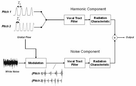
Figure 4.1 Pitch modification model.
Recall the waveforms generated
in synthesizing a vowel signal, :
|
|
|
(4.5)
|
The periodic portion of voiced speech is represented by
the expression ,
where is the impulsive excitation spaced by a pitch
period to a chain of linear time-invariant filters with impulse responses ,
,
and .
These filters represent the glottal waveform shape, vocal tract acoustic
filter, and radiation characteristic, respectively. The aperiodic or noise
portion of voiced speech is represented by the expression ,
where is the stochastic excitation to the same
filters and ,
being the multiplicative modulation function
and .
The pitch modification system developed in this study is
non-parametric and estimates the envelope of the estimated noise source without
assuming a specific shape for the envelope. In addition, the inherent speech noise
is not re-synthesized with an arbitrary white Gaussian noise source (as was
done by Stylianou et al. [43, 74, 75]). To approach the problem of
accurate pitch modification, we attempt to reverse-engineer the physiological
pitch modification model of Figure
4.1. A diagram outlining our pitch-scale modification
algorithm is shown in Figure
4.2.
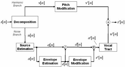
Figure 4.2 Block
diagram of approach to pitch-scale modification.
The aim of the Decomposition block is to reverse the summation
step and decompose the signal into periodic and noise components. With this
decomposition, any changes made to the periodic portion of speech can be
balanced by modifications in the aspiration noise component. We denote the
input speech signal as ,
and the harmonic and noise estimates from the Decomposition block and ,
respectively.
The flow diagram then splits the processing stages into two
branches: the Harmonic Branch and the Noise Branch. In the Harmonic Branch,
standard techniques can be applied to scale the pitch of the harmonic component
estimate. The harmonic component at the new fundamental frequency, ,
is then summed to the modified noise component, .
This additive model is identical to the vowel production model of Figure 2.3.
The Noise Branch in Figure
4.2 warrants more complex signal processing. To preserve
temporal synchrony between traits of the periodic and noise sources (see
discussion in Section 2.6), a mechanism is designed to estimate the aspiration
noise source from the aggregate noise component estimate, .
Algorithms that would usually be applied in a one-step Pitch Modification block,
as in the Harmonic Branch, would not work in the Noise Branch. These algorithms
traditionally need to be able to compute correlations for pitch determination,
which is prohibitive in white noise signals. Thus, complexity is added to
modify the noise component in the Noise Branch.
Modification of the aspiration
noise source is accomplished by first removing the spectral effects of the
vocal tract filter and radiation characteristic in the Source Estimation block.
The output signal, ,
can be viewed as the source estimate from the aspiration noise signal, .
For instance, if a linear filter with impulse response were designed for this block, we would utilize
the following equation:
|
|
|
(4.6)
|
The result is an estimate of the aspiration noise
source, which is related to the noise source waveform, .
The waveform, ,
thus has features of a white noise signal with a modulation function imposed on
it. Since modifying the fundamental frequency of the harmonic component
involves shifting the time instances of glottal excitation (recall Section 4.1), and since the noise component contains modulations
that occur at certain times within the glottal cycle (recall Section 3.5), the noise modulations must be modified in the same
manner. The approach we take is to de-modulate and re-modulate the noise source
with a new modulation function scaled by the pitch modification factor.
The Envelope Estimation block computes
,
a waveform related to the glottal flow waveform (recall the coupling between
the two sources in Figure
4.1). With the modulation function computed, we divide
out the effect of the envelope to result in an estimate of the de-modulated
white noise estimate, :
|
|
|
(4.7)
|
The remaining intermediate
waveforms in our flow diagram are “prime” versions of waveforms described so
far. The “prime” indicates that the waveform is at the new fundamental
frequency. The Envelope Modification block in Figure
4.2 changes the rate of the modulation function so that modulations
in the noise source are now synchronized with the modified harmonic component, .
The new envelope, ,
is a pitch-scaled version of .
The modified aspiration noise source, ,
is derived from the de-modulated noise source and the new envelope to generate
the new aspiration noise source, :
|
|
|
(4.8)
|
This new source is then
filtered by the inverse of to represent the vocal tract resonance
properties and radiation characteristic. The impulse response, ,
is convolved with the new aspiration noise source to produce the pitch-modified
version of the aspiration noise component, :
|
|
|
(4.9)
|
The overall pitch-modified
speech signal, ,
is then re-synthesized by adding the modified harmonic and noise components:
|
|
|
(4.10)
|
Section 4.5 next describes the implementation of this approach to
pitch modification and discusses the selection of specific algorithms.
4.5
Implementation of
Proposed Pitch-Scale Modification
As mentioned above, the proposed approach to pitch modification
essentially attempts to reverse-engineer the pitch modification model to modify
the aspiration noise source characteristics. The following sections describe
implementation of each block in Figure
4.2.
The
output of the PSHF method by Jackson and Shadle [31] is
used as the first stage in the pitch modification algorithm. Implementation of
the PSHF method was described above in Section 3.2. The outputs of the PSHF method used in the pitch
modification algorithm are chosen to be the outputs after spectral
interpolation, and for the harmonic and noise component
estimates, respectively. The reconstructed harmonic component is sent through
the Harmonic Branch, and the reconstructed noise component passes to the Noise
Branch in the modification scheme of Figure
4.2.
Pitch modification of the harmonic component estimated by the
PSHF algorithm can be accomplished by any of the algorithms introduced in
Section 4.1. The drawbacks of many of the methods are
circumvented if they are used to process only the periodic component of a
vowel. We implemented our own version of TD-PSOLA in MATLAB [47] for a simple modification
scheme that we will consistently use. The TD-PSOLA is diagrammed in Figure 4.3 and involves the following steps (from [54]):
1) Determination of analysis pitch marks.
These are times of the time instants of glottal closure that must be
determined. The Praat speech analysis tool [4] is used to estimate the
analysis pitch marks.
2) Formation of short-time segments. Each
segment is formed by a Hanning window centered on the analysis pitch marks and
two pitch periods in length.
3) Determination of synthesis pitch marks.
The first synthesis pitch mark is fixed to be at the same time as the first
analysis pitch mark. The next synthesis pitch mark is located one pitch period
away, where this pitch period is derived from the new local pitch. For
simplicity, the pitch modification factor is constant across the entire speech
segment, and the pitch contour is modeled to be piecewise-constant.
4) Mapping of analysis windows to synthesis
pitch marks. At each synthesis pitch mark, an analysis frame is inserted. In
the case of pitch decreases, an analysis frame may not be associated with a
synthesis pitch mark and thus discarded. Likewise, when increasing the pitch, analysis
frames may be replicated at more than one synthesis pitch marks. See Figure 4.4 for a schematic of how analysis frames are chosen.
5) Overlap-add synthesis. The short-time
segments at the new pitch are merged together.

Figure 4.3 Block diagram of TD-PSOLA algorithm.
|
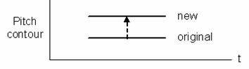
(a)
|
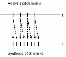
(b)
|
Figure 4.4 Example schematic of TD-PSOLA algorithm,
pitch scale = 2. (a) Original and new pitch contours and (b) replication of analysis
frames centered at glottal closure instants.
The TD-PSOLA method is less practical on stochastic speech
sounds since pitch estimators (e.g., autocorrelation techniques [4] or frequency-domain
peak-picking [65]) cannot estimate a modulation
rate in the aspiration noise source. Consequently, the proposed pitch
modification algorithm treats the noise component output of the PSHF differently
from the periodic component estimate. Pitch modification of the noise branch in
the algorithm (Figure
4.2) is described in the next section.
The crux of the algorithm lies in the processing of the noise
component estimated by the Decomposition block Figure 4.2. The Source Estimation stage obtains an estimate of the
noise source itself. In other words, inverse filtering is performed prior to
envelope estimation so that modulations in the aspiration noise may be modified
as they appear prior to vocal tract filtering.
Source Estimation
The Source Estimation block estimates the underlying source
waveform. Joint estimation algorithms could be inserted here, in which the
decoupling of source and filter is not assumed [32]. We choose, on the other
hand, the linear source-filter assumption of speech production, utilizing
linear prediction analysis to remove the effects of the linear time-invariant
filters and (recall Figure
2.3). It is tempting to estimate the modulation function,
,
by only inverse filtering by the periodic component of speech, .
In this case, however, the result would approximate the derivative of the
glottal waveform, ,
and make it impossible to estimate the DC component of the glottal airflow
waveform.
Instead, recall that the aspiration noise estimate is modeled by
.
We then estimate the modulation function, ,
so it may be modified and re-imposed on the noisy excitation waveform, .
The immediate goal of the Source Estimation stage is to analyze the noise
component estimate, remove the effects of the filters and ,
and estimate .
The choice of using linear prediction to estimate the
aspiration noise source requires several assumptions. Wide-sense stationarity
(WSS) is a constraint for linear prediction to be effective; therefore analysis
must be performed on short-time frames of the aspiration noise estimate. Since WSS
implies that the mean and variance of the underlying random process are unchanging,
the duration of the windowed frame must be short enough to ensure WSS but long
enough to afford a fair amount of spectral resolution.
After the whitening computation, it is assumed that any
modulations in the resulting white noise are preserved. Implied by linear
predictive analysis is that the linear filters acting on the stochastic process
are of all-pole forms. The all-pole assumption is valid for many voiced sounds,
except for nasals, which are produced with a closed side branch at the mouth
and excessive losses due to the compliance of the nasal passage walls [73]. The all-pole assumption also
does not adequately handle the radiation characteristic, which was modeled as a
single zero from the first-difference filter in Equation (2.10). Our use of linear predictive analysis relies on the
fact that this single zero may be approximately modeled by several poles [63].
Whitening of the input signal, ,
is implemented as follows. Overlap-add analysis utilizes a 20-ms Hanning
analysis window (length ) with half-window overlap:
|
|
|
(4.11)
|
where is the frame number, is the frame advance, and is the Hanning window in Equation (3.1). See Appendix E for a derivation of the inverse filter, ,
using linear prediction analysis of stochastic signals. The th inverse filter is applied to the th windowed frame, :
|
|
|
(4.12)
|
We can reconstruct the entire source
estimate from the short-time segments using overlap-add synthesis [63]:
|
|
|
(4.13)
|
where is the number of segments. Note that the
normalization factor takes into account the weighting effects of the analysis
and synthesis windows.
Figure
4.5 displays an example case of the whitening process
performed on the aspiration noise component of a synthesized /a/ vowel. The
aspiration noise source is either modulated with the glottal waveform or unmodulated.
When modulated, function is at a constant 100-Hz rate. As desired, the
whitening process approximately preserves the time-domain modulation
characteristics of the aspiration noise source.
|
(a)
|
(b)
|
Figure 4.5 Inverse filtering the noise component estimate
of a synthesized vowel. Whitened noise estimate plotted where the synthesized aspiration
noise source was either (a) modulated or (b) unmodulated. Synthesis parameters:
Noise type = modulated, Vowel = a, f0= 100, Gender = m, fs = 8000, Duration = 1,
DC = 0.1, OQ = 0.6, HNR = 10.
Envelope Estimation
The result of the Envelope Estimation block in Figure 4.2 uncovers the noise modulations generated by the
glottal airflow undulations. In other words, armed with an estimate of ,
envelope detection can estimate the modulation function, .
We have chosen a method based on the Hilbert transform. (See Appendix F for a comparison of two envelope detection methods.)
The Hilbert transform method is schematized
in Figure
4.6. The discretized estimate of the aspiration noise
source, ,
is related to the output envelope, by:
|
|
|
(4.14)
|
where is the discrete impulse response of the
quadrature filter in Figure
4.6 and is a 50-tap finite impulse response low-pass filter
with a 3-dB cutoff frequency set as a parameter of the algorithm (see parameter
list in Appendix A).

Figure 4.6 Hilbert transform method of envelope
detection, in continuous time. is the frequency response of the quadrature
filter that outputs the Hilbert transform of the input real signal. The complex
analytic signal is then formed, with its real part equal to and its imaginary part equal to its Hilbert
transform. Next, the magnitude of the analytic signal is taken. Finally, a
low-pass filter acts on the signal.
Envelope Modification
After uncovering the envelope of the noise source estimate, ,
the algorithm re-modulates the glottal noise source with a new scaled envelope.
To perform this envelope modification in our preliminary work, resampling was
performed on the envelope of the whitened modulated noise signal [50]. This method, however, was
only applicable to pitch scale factors less than one. To also provide for pitch
increases, the TD-PSOLA technique detailed above in Section 4.5.2 is used.
Dividing out the envelope from
the noise source estimate, we obtain the demodulated signal, :
|
|
|
(4.15)
|
The new envelope, ,
is then imposed on to form a modified source signal:
|
|
|
(4.16)
|
Spectral Coloring
The Spectral Coloring block re-imposes the spectral effects of
the vocal tract and the radiation characteristic on the aspiration noise
source. In the process of pitch modification, the pitch scale only affects the
source characteristics, while the movements of the speech articulators are
assumed unchanged. This assumption stems from the model of a decoupled voicing
source and vocal tract filter.
The input to the block is the
modified aspiration noise source, ,
and the output is its spectrally-shaped version, .
The newly-modulated white noise component, ,
is filtered by the radiation characteristic filter and an all-pole vocal tract
filter model with filter coefficients taken from the short-time segments chosen
in the Source Estimation stage. Overlap-add analysis results in the short-time
segments, :
|
|
|
(4.17)
|
where is the frame length, is the frame number, is the frame advance, and is the Hanning window from Equation (3.1).
The processing stage to obtain
the spectrally-colored short-time segment, :
|
|
|
(4.18)
|
where the vocal
tract/radiation filter, in the z-domain, ,
is
|
|
|
(4.19)
|
and the coefficients, ,
are taken from the th frames in the Source Estimation stage.
Overlap-add synthesis eliminates
the index and completes the reconstruction of :
|
|
|
(4.20)
|
where is the number of short-time segments, and
normalization is included due to both analysis and synthesis window weightings.
Finally, the modified aspiration noise, ,
is then summed with the modified harmonic component, ,
to yield the output at the new pitch, .
Three parameters are defined for the pitch modification algorithm: pitch scale,
LPC order, and LPF cutoff. The pitch scale indicates the constant ratio by
which the original pitch contour is multiplied. For example, a pitch scale of
1.2 indicates a pitch increase by a factor of 1.2. For a vowel with a
time-varying pitch linearly increasing from 100 to 120 Hz, the algorithm would
modify the pitch contour to 120144
Hz. The LPC order refers to the number of linear prediction coefficients to be
used in the Source Estimation stage ( in Appendix
E). The LPF cutoff is the 3-dB frequency
parameter of the low-pass filter in the Envelope Estimation stage of Figure 4.6. (See Appendix A for a tabulation of the modification parameters and Appendix
B for a MATLAB GUI that integrates the algorithms into
a visual representation.)
In Sections 3.3 and 3.4, we presented sample analyses on synthesized and real
vowels. These same vowels are now input into our pitch-scale modification
algorithm. The goal is to appropriately modify both the fundamental frequency
of the periodic component of speech and any modulations in the aspiration noise
source.
Steady Pitch
Figure
4.7 and Figure
4.8 step through the process of pitch modification using
the new algorithm. Figure
4.7 displays the block diagram of the algorithm with
unique letters indicating the waveform resulting from a specific stage in
processing. These letters correspond to the waveform labels in Figure 4.8. Synthesis parameters are: Noise type = modulated,
Vowel = a, f0 = 100, Gender = m, fs = 8000, Duration = 1,
DC = 0.1, OQ = 0.6, HNR = 10. Modification parameters are: Pitch scale = 0.8,
LPC order = 10, LPF cutoff = 350. The salient parameters are the input pitch
and the pitch scale. The pitch of the input synthesized vowel is 100 Hz, static
across the entire signal. The output waveform is a pitch-modified version of
the input, where the pitch scale is equal to 0.8, indicating a desired pitch of
80 Hz at the output.
Each step breaks down the signal into its constituent
components, allowing for specific analysis of the aspiration noise source. The
underlying assumption to be kept in mind is that the pitch change of an
individual only affects the source characteristics at the glottal level of the
speech production system. As a result, pitch modification of aspiration noise
must solely modify the aspiration noise source waveform. This is the critical
processing stage. Before- and after-modification waveforms of the aspiration
noise source are displayed in Figure
4.8g and h, respectively.
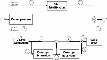
Figure 4.7 Block diagram for pitch modification
example. Letters denote the speech waveform at a specific instance during
processing. (a) Synthesized vowel, (b) modified vowel output, (c) extracted
harmonic component, (d) modified harmonic component, (e) extracted noise
component, (f) modified noise component, (g) aspiration noise source estimate,
(h) modified aspiration noise source, (i) envelope of aspiration noise source,
(j) modified envelope, and (k) demodulated aspiration noise source.
Figure 4.8 Pitch modification example, synthesized
vowel. Original and modified waveforms are placed side-by-side for ease of
comparison. (a) Synthesized vowel, (b) modified vowel output, (c) extracted
harmonic component, (d) modified harmonic component, (e) extracted noise
component, and (f) modified noise. See Figure
4.7 for the waveform’s location in the algorithm (letters
correspond to waveforms in this figure). Synthesis parameters: Noise type =
modulated, Vowel = a, f0 = 100, Gender = m, fs = 8000,
Duration = 1, DC = 0.1, OQ = 0.6, HNR = 10. Modification parameters: Pitch
scale = 0.8, LPC order = 10, LPF cutoff = 350.
Figure 4.8
continued… Pitch modification example, synthesized
vowel. Original and modified waveforms are placed side-by-side for ease of
comparison. (g) Aspiration noise source estimate, (h) modified aspiration noise
source, (i) envelope of aspiration noise source, (j) modified envelope, and (k)
demodulated aspiration noise source. See Figure
4.7 for the waveform’s location in the algorithm (letters
correspond to waveforms in this figure). Synthesis parameters: Noise type =
modulated, Vowel = a, f0 = 100, Gender = m, fs = 8000,
Duration = 1, DC = 0.1, OQ = 0.6, HNR = 10. Modification parameters: Pitch
scale = 0.8, LPC order = 10, LPF cutoff = 350.
This example involved pitch modification of a synthesized vowel,
where we have access to all waveforms that serve as building blocks for the vowel.
Comparisons of waveforms at the various stages of the pitch modification
algorithm may be made with waveforms from the stages of vowel synthesis. The
idea of reverse-engineering the model has already been mentioned, and its
benefits are evident here. The example stepped through in Figure 4.8 can be viewed from a synthesis point of view. To
simulate the decrease in pitch from 100 Hz to 80 Hz, we can simply synthesize
two vowels with fundamental frequencies of 100 Hz and 80 Hz, respectively. We
can compare waveforms from the synthesized vowels with the waveforms during
each stage of processing in the pitch modification algorithm.
Figure
4.9 shows the vowel production model with labels
indicating waveforms at each stage of vowel synthesis. Corresponding waveforms
at each stage of synthesis for different-pitched vowels are displayed side by
side in Figure 4.10. The left waveforms are from the 100-Hz vowel, and
the right waveforms are from the 80-Hz vowel. The general characteristics of
the modified noise and source waveforms are preserved. Compare Figure 4.8e, f with Figure
4.10e, f. However, the corresponding envelopes (compare Figure 4.8i, j with Figure
4.10i, j) differ due to the stochastic nature of the
envelope in the presence of aspiration noise. (See discussion in Section 5.1.3).
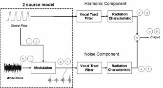
Figure 4.9 The vowel production model with labels at
each stage. Letters denote the speech waveform at a specific instance during
processing. At each step, the first letter indicates vowel synthesis at one
pitch; the second letter indicates vowel synthesis at another pitch. (a, b)
Synthesized vowel, (c, d) harmonic component, (e, f) noise component, (g, h)
aspiration noise source, (i, j) envelope of aspiration noise source, (k, l)
aspiration noise source before modulation.
Figure 4.10 Vowel synthesis of two vowels, simulating a pitch
change from 100 Hz to 80 Hz. (a, b) Synthesized vowel, (c, d) harmonic
component, and (e, f) noise component. See Figure
4.9 for the waveform’s location in the algorithm (letters
correspond to waveforms in this figure). Synthesis parameters: Noise type =
modulated, Vowel = a, f0 = 100, Gender = m, fs = 8000,
Duration = 1, DC = 0.1, OQ = 0.6, HNR = 10.
Figure
4.10 continued… Vowel
synthesis of two vowels, simulating a pitch change from 100 Hz to 80 Hz. (g,
h) Aspiration noise source, (i, j) envelope of aspiration noise source, (k, l)
aspiration noise source before modulation. See Figure 4.9 for the waveform’s location in the algorithm (letters
correspond to waveforms in this figure). Synthesis parameters: Noise type =
modulated, Vowel = a, f0 = 100, Gender = m, fs = 8000,
Duration = 1, DC = 0.1, OQ = 0.6, HNR = 10.
Time-varying Pitch Contour
We analyzed and decomposed a vowel into its harmonic and noise
components in Figure 3.8 above, which was synthesized with a linearly increasing pitch
from 100 to 140 Hz over one second. We now apply our pitch modification
algorithm to scale the pitch by a fixed factor of 1.2, shifting the endpoints
of the contour to 120 and 168 Hz. Figure
4.11 displays a wideband spectrogram of the pitch-modified
vowel along with the original and modified pitch contours. An autocorrelation
pitch estimation technique [4] was used to compute pitch values
every 5 ms.
Figure 4.11 Synthesized vowel with time-varying pitch,
100-140 Hz, over one-second duration, shown in Figure 3.7. (a) Wideband spectrogram and (b) original (dotted
line) and modified (solid line) pitch contours. Synthesis parameters: Noise
type = modulated, Vowel = a, f0 = 100140,
Gender = m, fs = 8000, Duration = 1, DC = 0.1, OQ = 0.6, HNR = 10. Modification
parameters: Pitch scale = 1.2, LPC order = 10, LPF cutoff = 350.
Figure 4.12 displays the modified components of the vowel, and Figure 4.12c indicates that the TD-PSOLA algorithm works effectively
on the harmonic component to decrease the original pitch periods. A 0.1-s
sample waveform of the modified envelope is displayed in Figure 4.12a, superimposed on the modified noise source waveform.
The modified noise component, re-constructed by applying spectral coloring due
to the vowels formants, is displayed in Figure
4.12b.
The desired synchrony is that maxima in the noise source
envelope occur during the open phase of the glottal waveform. To observe this
property, the modified envelope is superimposed as a dotted line on the
modified periodic waveform in Figure
4.12c. The peaks in the modified envelope function lie
just prior to the instants of glottal closure, during the open phase of the
glottal cycle. An advantage of the modification algorithm is its approximate
preservation of the original synchrony between the noise source modulations and
the periodic component.
Figure 4.12 Modified components of synthesized vowel. (a)
Modified aspiration noise source with modified envelope (dotted line), (b)
modified noise component, and (c) modified periodic component with modified
noise source envelope (dotted line).
Normal Speaker
Recall that the spectrogram and waveform of
the syllable /pæ/ were displayed in Figure
3.9. Again, we apply our modification algorithm to scale
the pitch by 0.8. The spectrogram and input and output pitch contours are
displayed in Figure 4.13, indicating the change in fundamental frequency from
about 100 to 80 Hz. Further temporal analyses are performed as was done in
Section 4.6.1. Waveforms of the newly modulated noise source,
modified noise component, and modified harmonic component are displayed in Figure 4.14 for a 0.1-s time range. Recall that in the separated
aspiration noise component, Figure
3.10 showed that noise bursts appeared at instants of assumed
glottal closure (see Appendix D for glottal closure assumption). Synchrony between
the modified components is consistent with this observation. Figure 4.14c illustrates the synchrony by superimposing the
modified noise source envelope on the modified periodic component.
Figure 4.13 Utterance
by normal speaker, /pæ/, as in Figure
3.9. Pitch scale = 0.8. (a) Wideband spectrogram and (b)
original (dotted line) and modified (solid line) pitch contours.
Figure 4.14 Modified
components of normal speech. (a) Modified aspiration noise source with modified
envelope (dotted line), (b) modified noise component, and (c) modified periodic
component with modified noise source envelope (dotted line).
Pathological Speaker
We introduced the sustained /a/ vowel by the
pathological speaker in Figure
3.12. The patient was diagnosed with vocal fold cysts and
constricted structures in the laryngeal region. To compensate for his weaker
voice, the patient “hyperfunctioned” by forcing larger volumes of air through
the vocal apparatus.
Recall that we observed maximum amplitudes
in the envelope of the estimated aspiration noise source occurring at both the
assumed glottal open phase and the glottal closure instant. The modified
envelope should aim to preserve the synchrony of the original harmonic and
noise components. Figure
4.16 steps through the reconstruction of the modified
noise component using our algorithm. The envelope of the whitened noise signal
shows the relatively variable nature of the modulations in the pathological
vowel. It is then instructive to view the modified harmonic waveform along with
the envelope of the modified noise source. Some amplitude maxima in the
envelope coincide with the assumed open phase of the periodic component, but
other maxima occur at other phases within the glottal cycle. This possibly
illustrates the various source mechanisms of aspiration noise during phonation
when uttered by a speaker with vocal fold pathology.
Figure 4.15 Vowel by speaker
with voice disorder, as in Figure
3.12. Pitch scale = 0.9. (a) Wideband spectrogram and (b)
original (dotted line) and modified (solid line) pitch contours.
Figure 4.16 Modified
components of disordered speech. (a) Modified aspiration noise source with
modified envelope (dotted line), (b) modified noise component, and (c) modified
periodic component with modified noise source envelope (dotted line).
4.7 Observations on Signal Quality
Ultimately,
we are interested in judging aurally the signal quality of the proposed
approach against standard methods outlined in Section 4.1. Such an evaluation, including judgment of the
naturalness of the aspiration component, and how it is perceived to blend with
its corresponding periodic component, requires a rigorous listening test that
is beyond the scope of the current effort. Nevertheless, our informal listening
shows promise for the technique for a variety of pitch-scale factors and
synthesized vowels with steady and varying pitch contours, as well as for real
vowels. In these modified signals, the periodic component was altered by either
TD-PSOLA or by a sinewave-based approach [64, 65],
and the noise component was modified by our proposed method. For these signals,
we observed that the pitch-modified aspiration noise typically reflects the
aspiration in the original signal and suffers less from artifacts of the two
implemented standard techniques, such as those due to voicing errors in the
sinewave-based approach and glottal-closure estimation errors in TD-PSOLA.
Further discussion of a future study in the context of continuous-speech
processing and its extension to a more rigorous evaluation are given in Section
5.1.5.
Chapter 4 presented an alternative strategy to pitch-scale
modification that aims to preserve temporal characteristics in the aspiration
noise source that were observed in the analysis of Chapter 3. Inspired by the physiology of pitch change in speech
production, the proposed strategy took a dual processing approach to pitch
modification. The harmonic and noise components of the speech signal were
separately analyzed, modified, and re-synthesized, so that temporal synchrony
was approximately maintained between the sources of each component. Current
algorithms take different approaches to implementing pitch modification. Some
process the signal as a whole, while others first obtain an estimate of the
source before modifying the fundamental frequency. Some function in the
spectral domain, while others operate on time-domain waveforms. None, however,
addresses temporal synchrony between the periodic and noise source signals.
The proposed approach is a non-parametric
analysis and modification strategy that does not assume any specific modulation
pattern such as in the noise modulation model. The TD-PSOLA method was selected
to modify the harmonic component of speech because of its high time resolution
properties and its relative success in perceptual quality. Due to the modeled
coupling between the harmonic and aspiration noise components, processing the
noise component was more involved. Modification of the fundamental period of
the periodic component was balanced by modifications in the temporal features
of the noise component. Although our vowel production model assumed one type of
noise source modulation, decomposition of real vowels demonstrated that noise
bursts seem to appear in more than one phase of the glottal cycle.
The algorithm’s implementation and
parameters were described in Section 4.5, and example cases of pitch-scale modification were presented
in Section 4.6. Results are promising, providing evidence that our
algorithm appropriately analyzes the aspiration noise component and attempts to
preserve noise modulations in the modified speech signal.
Chapter 5
This thesis concludes with a look into improving the algorithms
of the current study. The following sections discuss possible ways and take
initial steps toward adding robustness and flexibility to the vowel synthesizer
of Chapter 2, the harmonic/noise analysis algorithm of Chapter 3, and the pitch-scale modification strategy of Chapter
4.
Section 5.1.1 introduces the perturbation effects of jitter and
shimmer that are ubiquitous in running speech and extends the synthesizer
flexibility to include these parameters. The effects of the perturbations on
the performance of the separation algorithm are discussed. As a result, Section
5.1.2 presents the possible advantages of SEEVOC [61], an alternate strategy for
resolving the periodic portion of speech when perturbations are present.
Section 5.1.3 discusses the issues inherent in estimating a
modulation function from a broadband stochastic carrier signal. Section 5.1.4 challenges our pitch modification model in Figure 4.1, which assumed a strict decoupling between the
control of fundamental frequency and formant resonances in the vocal tract.
Finally, Section 5.1.5 and 5.1.6 present preliminary investigations into extending the
developed algorithm to process continuous speech and provide future directions on
perceptual ratings of different algorithms.
When observing the results from both normal and disordered
voices, often the analysis of the aspiration noise component is confounded by
perturbations to the signal other than randomness due to aspiration noise
sources. In the PSHF decomposition algorithm, the noise component is simply
assumed to be the residual after stripping the speech waveform of its estimated
harmonic component. In the residual, aspiration noise is a major contribution,
but so are the effects of frequency jitter and amplitude shimmer. These
perturbations may have their root in physiological mechanisms of neural or
muscular origin. Currently, the decomposition algorithm can handle low levels
of these perturbations while still performing adequately. Refinement and
extension of the algorithm to eliminate the jitter and shimmer influences in
the aspiration component estimate is a goal of future research.
To illustrate the jitter/shimmer issue, implementation of the
vowel production model was extended to allow synthesis of perturbed source
components. A common measure of jitter is its percent deviation from the
nominal pitch period value. During synthesis, the glottal flow waveform is
generated during each pitch period and concatenated with successive waveforms.
Recalling that the duration of the cycle corresponds to the pitch period ,
we have control over the period of each cycle in the synthesized vowel. For
example, we can modify the synthesis of a steady-pitch vowel by adding jitter
and shimmer into the pitch period parameter.
During each glottal cycle, the nominal
pitch period, ,
is perturbed using the following equation (from [31]):
|
|
|
(5.1)
|
where is the maximum jitter percentage and is a random variable with uniform distribution
between 0 and 1. The factor serves to transform the uniform random
variable into one with zero mean and extremes dependent on the maximum jitter
percentage parameter. Similarly, shimmer is applied as a cycle-to-cycle
variation in the amplitude of the source excitation. The equation for each
cycle’s perturbed amplitude, ,
is
|
|
|
(5.2)
|
where is the maximum jitter percentage and is the random variable defined above.
To observe the individual effects of jitter and shimmer, PSHF separation
of harmonic and noise components is performed on a synthesized vowel with HNR =
dB (idealized as a voiced source with no
aspiration noise energy). Synthesis parameters are listed in the caption of the
following illustrative figures. Figure
5.1 displays the extracted aspiration noise component
when the input vowel was synthesized with a maximum jitter percentage of 1%.
The percept of the vowel is one of slight roughness. A sampling rate of 48000
Hz is chosen to minimize undersampling effects. Note that a significant, although
small, noise component has leaked into the output of the decomposition
algorithm. The current study assumes any output energy at this stage is due to
turbulent noise sources at the glottis. The result of the simulation in Figure 5.1 shows that a significant jitter contribution can
confound the subsequent pitch modification algorithm. The algorithm would
attempt to uncover modulations inherent in the aspiration noise component, even
though the signal itself is known not to be due to aspiration noise.
Figure 5.1 Noise waveform estimated from purely
periodic vowel with jitter. Synthesis parameters: Noise type = modulated, Vowel
= a, f0 = 100, Gender = m, fs = 48000, Duration = 1, DC =
0.1, OQ = 0.6, HNR = 500, jitter = 1, shimmer = 0.
Similar observations of non-aspiration noise sources leaking
into the extracted noise component are seen when adding a shimmer factor with
no jitter and aspiration noise contributions. Although not as much leakage is
observed for a 10% shimmer parameter (Figure
5.2), the result is still perceptible and can easily
degrade the performance of the pitch modification algorithm. With each
additional stage of processing, errors accumulate and can be potentially
magnified. Compensation for these perturbations warrants novel signal
processing techniques.
Figure 5.2 Noise waveform estimated from purely
periodic vowel with shimmer. Synthesis parameters: Noise type = modulated, Vowel
= a, f0 = 100, Gender = m, fs = 48000, Duration = 1, DC =
0.1, OQ = 0.6, HNR = 500, jitter = 0, shimmer = 10.
SEEVOC, standing for spectral envelope estimation vocoder, was
developed in the early 1980s for the low-bit rate coding field to provide for
an efficient method of parametrically representing the spectral envelope of
short-time speech segments [61]. Applications of the SEEVOC algorithm
include background noise estimation, noise suppression, and, most relevant to
this study, high-quality pitch estimation. For our purposes, we use the SEEVOC
algorithm to help handle jitter and rapid pitch changes that occur in voiced speech.
In the present PSHF algorithm, both stationarity and strict
harmonicity are assumed over the analysis window of four pitch periods in
duration. To estimate the signal’s harmonic component, the PSHF simply samples
the frequency spectrum at integer multiples of the local pitch estimate. Over
the duration of the analysis window, however, there may be deviations in the
frequency location of particular harmonics due to rapid fluctuations or more
subtle perturbations in the pitch period. This movement is effectively averaged
out when the discrete Fourier transform is taken. With such pitch fluctuations,
harmonic energy can lie at frequency bins of the DFT other than bins that are
harmonically spaced apart. In a way, a pseudo-harmonic filter could be applied
to determine the energy attributed to the periodic component, and this is what
SEEVOC attempts to do.
The SEEVOC algorithm models the periodic source as an impulse
train that is filtered by the spectral properties of the vocal tract
resonances. In the spectral magnitude domain, this model dictates that the
envelope is sampled by line spectra at integer multiples of the fundamental
frequency. The strictness of this spectral sampling assumption is relaxed.
Instead of blindly selecting the harmonic bins of the discrete Fourier
transform, SEEVOC uses frequency ranges centered on harmonic bins and looks to
the left and right of the bin by half the fundamental frequency. The algorithm
then utilizes a peak-picking technique within this range to determine the
spectral bins that correspond to the periodic source. Frequency errors are
avoided by bootstrapping each search from the previous frequency estimate. To
connect the dots of the spectrum, linear interpolation is performed in the log
frequency domain. Finally, a minimum-phase constraint is applied before
calculating the inverse DFT to yield the spectral envelope’s impulse response.
For our purposes, we can directly apply the SEEVOC algorithm up
to the final steps. Once the periodicity bins are identified from the magnitude
of the DFT, we can revert to the DFT’s complex coefficients and perform an
inverse DFT of the pseudo-comb filter to arrive at an estimate of the periodic
component. To reconstruct the aperiodic component due to the aspiration noise
source, we can take the inverse transform of the remaining frequency bins, or
first interpolate across the zeroed bins as was done in the PSHF method.
5.1.3
Estimating
the Envelope of a Noise Signal
One of the critical steps in the proposed pitch-scale
modification algorithm is Envelope Estimation in the Noise Branch of Figure 4.2. This stage estimates the slow-moving amplitude of
the modulated noise signal that represents the aspiration noise source. We
mentioned the magnitude of the analytic signal derived using the Hilbert
transform is known to reconstruct an envelope that was imposed on a narrowband
carrier signal. When imposed on a broadband signal such as white noise, the
reconstructed envelope results in a suboptimal estimate. Here, we briefly
explore the cause of this estimation difficulty.
As an example case, an aspiration noise source waveform is
synthesized with an assumed periodic source at a fundamental frequency of 100
Hz. This means that a white Gaussian noise signal is multiplied by the glottal
airflow velocity waveform. Short-time spectral and temporal features of these
waveforms are displayed in Figure
5.3. As expected, the spectrum of the periodic source
shows peaks at zero due to the DC offset and at multiples of 100 Hz. The
spectrum of the modulated noise source waveform is distinctly broadband in
nature and notably dominates the periodic component above about 1300 Hz. One
DFT was computed to estimate the noise spectrum, justifiably translating into a
high variance estimate that is not perfectly flat.
The challenge is how to reconstruct the imposed modulation
function from the modulated noise signal. The Hilbert transform method used in
our study gives this initial estimate. Recall that the magnitude of the
analytic signal is smoothed by a low-pass filter with a 3-dB cutoff frequency
of 350 Hz. The resulting envelope estimate is displayed in Figure 5.3 at a normalized amplitude with the known modulation
function. The AC structure and DC offset measures are qualitatively preserved,
though the gain fluctuates from period to period.
Further improvements for the Envelope Estimation stage are
warranted. It may be possible to develop a comb filter method, similar to that
done in the PSHF decomposition algorithm, where the bins of the comb are placed
at harmonics of the local fundamental frequency. Judging from the spectra in Figure 5.3, the comb filter would be ineffective on the
modulated noise source and better suited on the output of the first-pass
envelope estimate. Jitter and shimmer issues similar to those encountered when
processing the overall pressure signal will complicate the processing. Even
with an effective comb filter, energy above the 6th harmonic is
already lost in the envelope estimate’s spectrum. (See Appendix F
for more discussion on envelope estimation.)
Figure 5.3 Difficulty estimating an envelope from a
noise signal. (a) Short-time spectra, (b) waveforms, and (c) envelope waveforms
with normalized amplitudes. Line types indicate the glottal airflow velocity
(thick line), noise source modulated by glottal waveform (thin line), and noise
source envelope estimated by Hilbert transform method (dotted line). Synthesis
parameters: Noise type = modulated, f0= 100, fs
= 8000, DC = 0.1, OQ = 0.6, HNR = 10.
In this study, the classic decoupled source-filter theory is
assumed as the model for the production of vocalic speech sounds. In this view,
the vocal apparatus can independently control the frequency of vibrations of
the vocal folds and the shape of the supraglottal cavities. In addition, the
acoustic impedance of the glottal orifice is assumed to be much larger than the
impedance of the vocal tract, further supporting the decoupled theory [73]. As explained in the physiology
of pitch control in Section 4.2, the fundamental frequency of vocal fold oscillation
is largely due to the stiffness of the vocalis muscle and vocal fold tissue
density, where the stiffness can be modulated by external laryngeal muscles.
Thus, each vowel’s associated formants, dependent mainly on the position of the
tongue, can thus be realized at a continuous array of pitches.
In reality, though, this simple model has been shown to be
incomplete by several studies investigating the coupling effect of formant
frequencies and the frequency of vocal fold vibrations. Perhaps the best
evidence for coupling is found in studies that simply analyze vowel acoustics across
many speakers and languages of the world. Peterson, Barney, and Lehiste have
documented what is referred to as the “intrinsic pitch of vowels,” where high
and low vowels are observed to be produced with higher and lower pitches,
respectively [44, 62]. The difference in pitches vary
anywhere from 4 to 25 Hz, and the difference has been shown to be significant
across different languages and testing settings [79]. Though not a physiological
verification of source-filter coupling, the evidence that humans tend to
co-vary their pitch with vowel formants demonstrates the existence of a natural
coupling phenomenon.
Turning to the speech production of the singing voice, a
commonly cited predicament is how soprano vocalists sing a vowel in which the
first formant frequency (F1) is lower than the fundamental frequency. In this
case, the percept of F1 is nonexistent, since the spectral envelope due to the
vocal tract resonances is effectively sampled at integer multiples of the
fundamental frequency. Sundberg has shown that, at high pitches, soprano
vocalists alter their tongue position to match F1 to the fundamental frequency [76]. One possible cause given for
this formant matching phenomenon is the need for the vocalist to maximum his or
her vocal efficiency. Thus, placing F1 at the location of the desired pitch
will maximally amplify the energy at the fundamental frequency.
Finally, in an interesting study by Rothenberg, it was shown
that the amplitude of the vocal fold vibrations can be affected by changes in
the vocal tract acoustics [69]. Again, the effect was only
observed when the subjects, female professional vocalists, produced vowels at
pitches greater than 600 Hz. Briefly, the experimental setup consisted of a
Rothenberg mask [68], an electroglottograph (EGG),
and a cylindrical tube whose variable position could be controlled by a
electromechanical transducer. Within a trial, the subject sustained a vowel
while the tube was dynamically pushed to the lips and pulled away. Adding the
tube effectively increased the acoustic length of the vocal tract and forced a
downward shift in F1. Rothenberg analyzed the EGG signals and concluded that
the amplitude of the vocal fold vibrations was decreased during the times when
the tube extended the length of the vocal apparatus.
Again, detailed aerodynamic and mechanical measurements have
not been made yet on the extent to which formant frequencies and pitch co-vary.
The results of these studies, however, point to an alternative pitch
modification model that provides for constant feedback between the periodic
source waveform and the resonance properties of the vocal tract acoustic filter.
In the analysis above, sustained vowels and vowels with
time-varying pitch were the speech signals of interest. Taking a broader view,
we are interested in continuous speech. Toward this objective, we have
developed a preliminary pitch-scale modification system that handles both
voiced and unvoiced speech by processing voiced speech with our proposed system
and then concatenating unprocessed unvoiced speech with our pitch-modified
voiced speech.
Figure 5.4a displays the original and modified waveforms of
continuous speech spoken by a non-pathological female speaker. The utterance is
“As time goes by.” The pitch scale is set to 0.8 and the original and modified
pitch contours are shown in Figure
5.5. A signal comparison is made in Figure 5.4 between outputs from our proposed modification
algorithm and from the sinewave transformation system (STS) discussed in
Section 3.1 [64, 65]. Both algorithms adequately
modify the pitch contour by the desired ratio. Using STS, the noise component
is perceived as somewhat tonal and more perceptually separate from the periodic
component. Harmonicity in the narrowband spectrogram in the 11.25
s window above 2500 Hz is overestimated by the STS algorithm in Figure 5.4b. This effect is due to the degree of voicing index
that selects a boundary frequency between periodic and stochastic spectral
regions. In the time between 1 and 1.25 s, it appears that the degree of
voicing is overestimated and the perceived speech is removed of aspiration
noise.
The output signal from the proposed algorithm is perceived to contain
a breathier quality, consistent with the quality of the original waveform.
Specifically, the signal characteristics displayed in Figure 5.4c tends to preserve the fullband aspiration noise
features from the original signal. The signal modified with the proposed
algorithm is free of artifacts and discontinuities that may appear in standard
modification techniques. When performing preliminary analysis on running
speech, however, it is observed that the decomposed noise estimate sometimes
contain leakage from the harmonic components. This harmonicity in the noise
spectrum, also observed when decomposing isolated vowel waveforms, is also
perceptually significant. The time-varying nature of natural vowels, in
addition to the effects already mentioned regarding jitter and shimmer, may
contribute to the suboptimal performance of the separation technique because of
inaccurate pitch estimation. Possible solutions may employ more advanced signal
processing methods to help create perturbation-free waveforms and to better
estimate the pitch contour of continuous speech.
Figure 5.4 Comparing pitch-scale
modification algorithms. Utterance by a normal speaker saying: “As time goes
by.” (a) Original signal, (b) modified by STS, and (c) modified by our proposed
algorithm. Narrowband spectrograms (upper plot) and time-domain waveforms
(lower plot) plotted for each signal. Modification parameters: Pitch scale = 0.8,
LPC order = 10, LPF cutoff = 350.
Figure 5.5 Original (thick line)
and modified (thin line) pitch contours of continuous speech example in Figure 5.4. Pitch contours similar for outputs of proposed
algorithm and STS.
5.1.6
Formal Listening Evaluation
We have made informal listening observations in both Sections 4.7 and 5.1.5, indicating promise to our proposed modification
approach on both vowels and continuous speech. Formalizing the evaluation
procedure is a direction of future work. Perceptual ratings of pitch-modified
speech may be performed using the mean opinion score (MOS) as the quality
index. To determine the MOS, listeners rate the quality of the speech signals
pitch-modified by different algorithms. Listeners give each signal a quality
rating ranging from 1 to 5: (1) unsatisfactory, (2) poor, (3) fair, (4) good,
and (5) excellent [35]. The MOS is the arithmetic
mean of all the individual scores. This assessment would provide for a
statistical significant way of evaluating our algorithm against baseline
algorithms.
In this study, we approached the problem of high-quality speech
synthesis and pitch-scale modification in the context of vocalic speech sounds
containing an aspiration noise component. We first developed a vowel production
model that follows the classic linear source-filter speech model, in which both
a periodic and stochastic source excite the acoustic filter in the vocal tract.
Inspired by physiological observations, we assumed an additive model, in which
both speech sources are coupled together, so that the stochastic excitation, or
aspiration noise source, is temporally modulated by the periodic source
waveform due to gating of turbulent airflow by vocal fold vibrations. The
glottal airflow velocity waveform, modeled by the Rosenberg pulse [67], serves as the multiplicative
modulation function that acts on the aspiration noise source. Based on our
model, we implemented a vowel synthesizer allowing us to explore the salience
of these modulations, specifically revealing the importance of temporal
synchrony between noise bursts and the periodic glottal airflow waveform. This
is consistent with previous research on the perception of natural-sounding
vowel synthesis [20, 36, 66].
To estimate the actual patterns of the noise modulations in the
aspiration noise signal, we turned to signal processing algorithms that analyze
a speech signal and separate its periodic and noise components. After
qualitatively reviewing state-of-the-art algorithms and quantitatively
evaluating one in particular, we chose to use the pitch-scaled harmonic filter [31] because of its simplicity and
ability to approximately preserve temporal modulation features present in the
noise component of a synthesized vowel waveform. Due to the stochastic nature
of aspiration noise, the envelopes of the noise modulations could only be
estimated to a certain degree, but show varying levels and types of modulation
patterns in normal and pathological speakers. Results of our analysis on real
vowels indicate that noise bursts can occur at several time instants within the
glottal cycle. In particular, after estimating the source of a noise component,
we observed noise amplitude maxima during the open phase of the assumed glottal
cycle and at time instants around glottal closure.
Finally, to enhance the natural quality of pitch-scale
modification algorithms, we designed a strategy to take into account the
observed patterns of modulation and temporal synchrony between the harmonic and
noise components in a voiced speech sound. We showed that advanced modification
algorithms have taken several different approaches to altering the fundamental
frequency of a speech signal and that we aimed to take the effective parts from
each strategy to develop a more physiologically-based algorithm. Inspired by
the physiology of pitch control in human speakers, our approach was designed to
preserve temporal and spectral features in the original speech signal. Assuming
our vowel production model, a change in pitch affected the fundamental
frequency of the periodic source and the modulation function imposed on the
turbulent airflow sources. Thus, after separating the original signal into its
harmonic and noise components, we focused on maintaining the inherent qualities
of the noise by implementing a non-parametric processing structure that
estimated the envelope of the modulated noise source and re-modulated the
source with a pitch-modified version of the envelope. Due to an inverse
filtering stage by linear prediction and a noisy envelope estimation procedure,
certain assumptions and caveats must be satisfied before effectively making use
of the proposed algorithm. For the given examples, however, the reconstructed
modified signal was perceptually natural-sounding and gives promise and
direction toward a more accurate pitch-scale modification system.
Appendix A
|
Synthesis parameter
|
Units
(if applicable)
|
Possible values
|
Default value
|
Purpose
|
|
Noise type
|
|
unmodulated,
modulated
|
modulated
|
Indicates whether the noise source is
modulated by the periodic glottal waveform or not.
|
|
Vowel
|
|
i, e, ae, a, o, u
|
a
|
Indicates formant values. See Table 2.1.
|
|
f0
|
Hz
|
Any positive number
|
100
|
Pitch track for synthesized vowel.
|
|
Gender
|
|
m, f
|
m
|
Selects set of formant values. See Table 2.1.
|
|
fs
|
Hz
|
Any positive number
|
8000
|
Sampling rate
|
|
Duration
|
seconds
|
Any positive number
|
1
|
Duration of vowel
|
|
DC
|
|
Any rational number between 0 and 1,
inclusive
|
0.1
|
Only relevant if modulated noise is
chosen. This parameter controls the amount of noise during the closed phase. The
minimum flow at the open phase is increased depending on DC flow.
|
|
OQ
|
|
Any rational number between 0 and 1,
inclusive
|
0.6
|
The open quotient. Dictates the open
phase duration (OQ/f0) within a glottal cycle.
|
|
HNR
|
dB
|
Any rational number
|
10
|
Sets the harmonics-to-noise power ratio.

|
Table A.1 Parameters
of vowel synthesizer.
|
Modification parameter
|
Units
(if applicable)
|
Possible values
|
Default value
|
Purpose
|
|
Pitch scale
|
Hz
|
Any positive, rational value
|
0.8
|
Pitch modification factor. For example,
if the input pitch is 100 Hz, the output pitch will be equal to 0.8(100) = 80
Hz.
|
|
LPC order
|
|
Any positive whole number.
|
10
|
Indicates order of all-pole model in the
linear prediction analysis of the inverse filtering stage. P in Equation (E.2).
|
|
LPF cutoff
|
Hz
|
Any positive number
|
350
|
3-dB cutoff frequency for low-pass
filter used in the Envelope Estimation stage (see Figure 4.6).
|
Table A.2 Parameters
of proposed pitch-scale modification algorithm.
Appendix B
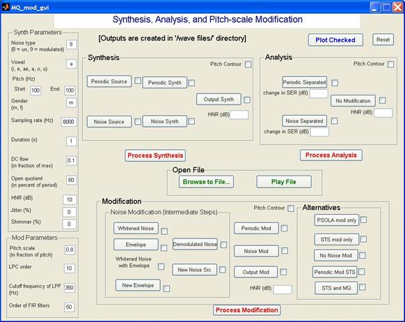
Figure
B.1 MATLAB GUI.
The parameters from the tables above were integrated into a
graphical user interface (GUI) in MATLAB [47] for rapid prototyping of
speech signal synthesis, analysis, and modification. A screen shot of the GUI
is displayed in Figure B.1. Chapter 2 discussed the background and development leading up
to the code behind the Synthesis GUI panel. Chapter 3 led the reader through the implementation behind the
Analysis panel that decomposes the input signal into harmonic and noise
components. Finally, Chapter 4 discussed the pitch-scale modification sections.
The GUI layout was designed for easy access to the waveforms
during intermediate processing stages of each algorithm. Each button can be
depressed to play the waveform out to the PC soundcard, and checkboxes are
available to select waveforms to be plotted. The left column allows user input
to control the parameters of vowel synthesis and pitch-scale modification. Note
that no parameters are needed for running the harmonic/noise decomposition
algorithm. In the future, it would be instructive to view the effects of
varying the analysis window duration. Presently, the embedded duration is fixed
at four times the local pitch period. Note that the harmonic-to-noise (HNR)
measures are calculated for the synthesized, analyzed, and modified signals to
allow for comparison of relative energy contributions. The “change in SER”
value is analysis performance measure from [31] that was not used in this
thesis.
In the Modification panel, alternative outputs are generated
that allow for analysis on the differences between different algorithms. In the
GUI, the overall signal is processed by the TD-PSOLA algorithm and the
sinusoidal transformation system (STS) based on the sinewave representation of
McAulay and Quatieri [64, 65]. In addition, No Noise Mod
refers to a modified output whose periodic component was modified using
TD-PSOLA and noise component was unmodified. Periodic Mod STS is a similar
waveform, except that the periodic component was processed using the STS
method. STS and MQ refers to a fusion of algorithms: the periodic component
being modified by STS and the noise component modified by the author’s proposed
approach from Section 4.4. Finally, Output Mod refers to the proposed
modification algorithm, in which the periodic component is processed by
TD-PSOLA and the noise component is modified as in our implementation (Section 4.5.3). Note also that intermediate steps in the proposed
pitch modification algorithm are identified and allowed to be plotted in the
GUI.
Finally, since our analysis encompasses both synthesized and
real vowels, the Open File button provides the ability for the user to access
any wave file containing a spoken utterance. In the case of the analysis of a
wave file, any changes to the synthesizer parameters are ignored and the
Synthesis panel outputs are meaningless. Processing can then be continued via
the Analysis and Modification panels. Microsoft WAV files are created for each
waveform and stored in a local “wave files” folder for easy access and
portability.
Appendix C
To gain insight into the pitch-scaled harmonic filter, we step
through the derivation for an example frame, where is the window length, is the sampling rate in Hz, and is the assumed pitch period, in seconds. We
start by knowing that the frequency spacing between bins of the -point DFT is Hz [60], which is the reciprocal of
the window duration, seconds. If is chosen to be an integer multiple of the
pitch period in samples, then we have ,
where is a positive integer. The DFT bin spacing, in
Hz, can then be written as .
Since the pitch, in Hz, is ,
each bin is spaced apart by of the pitch. For example, if is 4, the bin spacing would be one-fourth of the
pitch, and every fourth Fourier coefficient would contain power at harmonics of
the fundamental frequency.
Figure C.1 displays an example of a purely periodic vowel signal
and its analysis by the pitch-scaled harmonic filter. The vowel, with a steady
pitch of 100 Hz, has a pitch period length of 80 samples (fs = 8000
Hz). The factor is 4, and the 320-point DFT is taken of a
windowed segment of length 320 samples. The magnitude spectrum shows that the
harmonic energy is concentrated at every fourth DFT bin, a direct result of the
bin spacing being one-fourth of the pitch, or 25 Hz.
|
(a)
|
|
(b)
|
Figure C.1 Example of the pitch-scaled harmonic filter
on a windowed segment. (a) DFT of short-time signal from vowel signal in (b),
windowed by a Hanning window (dotted line). Circles in (a) indicate DFT magnitude
at every fourth DFT index. Synthesis parameters: Vowel = a, f0= 100, Gender = m, fs = 8000, DC = 0.1, OQ =
0.6.
Appendix D
Figure D.1 summarizes our definition of closed phase, open
phase, and glottal closure within a glottal cycle, or pitch period. The closed
phase is the time during which the membranous vocal folds are in contact and no
AC component exists. The open phase is the remaining duration of the pitch
period when airflow velocity is modulated by the vocal fold vibrations. The
glottal closure instant is the time when the open phase becomes the closed
phase. Note that the open quotient measure is the ratio between the open and
closed phases.
In our analyses in Sections 3.3, 3.4, and 4.6, we assumed that we could derive these properties of
the periodic source waveform by observing the pressure waveform of a vowel
after filtering by the vocal tract and radiation characteristics. The lower
waveform in Figure D.1 displays a vowel synthesized from the periodic source
in the upper waveform. The negative peaks in the filtered waveform correspond
with the instants of glottal closure. Deducing the open and closed phases from a
vowel waveform is difficult because of their relative closeness. However, we
can assume that samples just prior to the glottal closure instant are present during
the open phase of the source waveform.
Figure D.1 Defining glottal
waveform properties. Synthesized waveforms are of the periodic source (upper)
and corresponding vocal tract/radiation-filtered waveform (lower). Vertical
lines indicate instants of glottal closure. Synthesis parameters: Vowel = a, f0
= 100, Gender = m, fs = 8000, Duration = 1, DC = 0.1, OQ = 0.6.
Appendix E
Whitening is accomplished in each short-time segment by
estimating the all-pole filter that best fits the vocal tract resonance
properties and the radiation characteristic. Since the radiation characteristic
has a zero and behaves like a high-pass filter, the estimated poles model the
zero as closely as possible depending on the number of poles. The all-pole
model of a windowed aspiration noise waveform, ,
where the input is white Gaussian noise, ,
is displayed in Figure E.1.
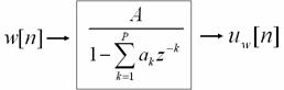
Figure E.1 All-pole model of aspiration noise.
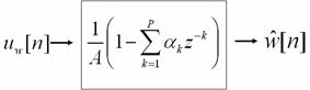
Figure E.2 The inverse approach to solving for the
all-pole model in the stochastic case.
Figure E.2 takes the inverse approach to solving for the
coefficients of the all-pole filter and rewrites the problem so that the filter
coefficients of a corresponding FIR filter are estimated to result in the best
estimate, ,
of white noise. Linear prediction of a stochastic signal can be used to find
these coefficients by assuming that each noise sample in the segment, ,
is predictable by a weighted sum of prior samples:
|
|
|
(E.1)
|
where is also the number of poles and values are the coefficients of the th-order filter, in the th frame. The error function, ,
minimizes the difference between the expected value of and the expected value of .
After minimizing the expected
value of the squared error by taking the derivative with respect to each coefficient, a set of equations in unknowns is obtained. The complete derivation
(see [63] for details) results in a th-order FIR filter whose coefficients are equal
to the ’s and the gain is .
We also fold in the inverted radiation characteristic filter to yield the
complete short-time inverse filter with impulse response, ,
and frequency response, :
|
|
|
(E.2)
|
Appendix F
Asynchronous AM Detection
In the communication systems world, a common method of
amplitude modulation (AM) detection is asynchronous envelope detection via a
diode rectifier and RC low-pass filter circuit. AM radio receivers further add
a DC block circuit so that the resulting envelope, the message of the signal,
can be played out over speakers [6]. A block diagram of
asynchronous envelope detection is displayed in Figure F.1.

Figure F.1 Classic method of asynchronous detection of
AM message. HWR = half-wave rectification, LPF = low-pass filter, -DC indicates
that the mean value is subtracted.
The form of AM signals is (from [6])
|
|
|
(F.1)
|
where denotes the modulation index or depth, is the message signal to be transmitted, is the unmodulated carrier signal amplitude,
and is the carrier signal’s frequency in rad/sec. The
carrier frequency must be much larger than the frequencies in the message
signal, so that the low-pass filter can effectively reject energy at the
carrier frequency while preserving the signal characteristics of the message.
Figure
F.2 shows an example of AM signal construction and the
output of the classic AM envelope detector. The message is composed of the sum
of two sinusoids at 10 and 17 Hz ( in Figure
F.2a), and the carrier signal is a 6000Hz
sinusoid ( in Figure
F.2b). The resulting AM signal is processed through the
stages in Figure
F.1. Figure
F.2d shows that the output of the envelope detector is
correct within a gain factor (about 6 in this case). For the application of AM
radio reception, this factor is not an issue since the gain can be controlled at
the receiver. (The modulation index, ,
in this case was set to 0.5, so its inverse does not make up the entire gain.)
The 3-dB cutoff frequency of the low-pass filter was set to 100 Hz and
implemented via a 50th-order finite impulse response filter.
Figure
F.2 Amplitude modulation example. (a) Message,
(b) carrier, (c) AM signal, and (d) envelope detected using asynchronous
detection (solid line), with desired envelope (dashed line).
As a second example to further test the asynchronous envelope detection
method, the same message was used as in the previous case in Figure F.3. The carrier frequency is decreased to 1000. The
resulting message signal does not follow the original message. The method is
not robust across different message, carrier, and LPF cutoff frequencies, and
this undesirable property prompts us to investigate the Hilbert transform
method.
Figure F.3 Amplitude modulation example with lower carrier
frequency. (a) Message, (b) carrier, (c) AM signal, and (d) envelope detected
using asynchronous detection (solid line), with desired envelope (dashed line).
Hilbert Transform Method
In the Hilbert transform method, the notion of an analytic
signal is introduced. Any real signal can be represented by its one-sided
Fourier spectrum due to its Hermitian symmetry, with an even magnitude and odd
phase characteristic. As a result, the spectral redundancy may be eliminated,
and the right side of the spectrum is termed the analytic representation of a
real signal [2]. The envelope of a real
signal may be calculated from its analytic representation through a
straightforward calculation. A derivation of the analytic signal follows (see [2] for details).
The analytic representation, ,
is equal to the sum of an original real signal, ,
plus a term, ,
derived from the Hilbert transform of the real signal:
|
|
|
(F.2)
|
The Hilbert transform, ,
is calculated by subjecting to a quadrature filter with impulse response .
The impulse response and frequency response, schematized in Figure F.4, are
|
|
|
(F.3)
|
where sgn(f) is the signum function (positive
frequencies retain their sign, while the phase of negative frequencies shift by
180°). Thus, the analytic signal is a complex function, its real part equal to
the original real signal, ,
and its imaginary part equal to .
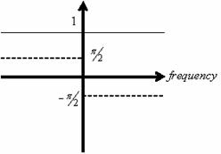
Figure F.4 Schematic of frequency response of the
Hilbert quadrature filter. Magnitude (solid line) and phase (dashed line)
response.
The spectrum of the analytic
signal, ,
is simply
|
|
|
(F.4)
|
where is the unit step function with .
The complex envelope, ,
of a real signal is derived from its analytic representation:
|
|
|
(F.5)
|
and the instantaneous amplitude, ,
of the real signal, ,
is then defined as
|
|
|
(F.6)
|
In the case of AM signal demodulation, is the AM signal, from Equation (F.1). Essentially, the Hilbert transform method computes
the magnitude of the analytic signal of a real signal. The analytic signal, ,
is simply
|
|
|
(F.7)
|
and the instantaneous
amplitude, ,
is
|
|
|
(F.8)
|
In the aspiration noise source
case, the carrier signal is white noise, ,
and the message signal is the glottal flow waveform estimate, .
Since the glottal flow waveform is assumed to always be greater than zero
(negative airflow is ignored), notation is transferred from that of AM to that
of DSB-SC (double side band-suppressed carrier). The “suppressed-carrier”
notation stems from the fact that the modulated signal, ,
eliminates the energy at the carrier frequency:
|
|
|
(F.9)
|
The modulation index, ,
disappears since the depth of modulation is dictated by the AC amplitude of the
message, .
A demodulation example with the same 1000-Hz carrier and message as before is
depicted in Figure F.5. As expected, the demodulated message matches the
modulating function.
Figure F.5 DSB-SC modulation example. (a) Message, (b)
carrier, (c) AM signal (solid line) with message (dashed line), and (d)
envelope detected using Hilbert transform method (solid line) with desired envelope
(dashed line). Note the lines in (d) are offset vertically by 0.2 for clarity.
Figure F.6 gives an envelope detection example with two
sinusoids modulating a white noise carrier. The demodulated signal is shown in Figure F.6d. The magnitude of the analytic signal seems to
follow each local peak of the DSB-SC signal instead of tracing the
low-frequency message signal. The result is expected since the Hilbert envelope
is known to work in the case of narrowband carriers.
Figure F.6 DSB-SC modulation example with noise carrier.
(a) Message, (b) carrier, (c) AM signal (solid line) with message (dashed
line), and (d) envelope detected using Hilbert transform method (solid line) with
desired envelope (dashed line).
To recover the low-frequency information, a low-pass filter is
appended to the Hilbert transform method in Figure
F.7. The cutoff frequency is chosen to be 100 Hz in the
example case and waveforms are re-displayed in Figure F.8. The estimated envelope better matches the desired
message signal, though the amplitude of the envelope does not match that of the
modulation function. The method reveals the modulation function better than the
AM envelope detector. In speech applications, we will assume that any relevant
modulation information exists below 350 Hz (an upper pitch limit for normal
adult pitch ranges). It is known that the envelope cannot be estimated exactly
when the carrier is a broadband signal such as white noise. The difficulty of
determining the envelope of a noise carrier is evident, but the Hilbert
transform method helps approximate time-domain modulations within the context
of inherent random ripples in the noise envelope.

Figure F.7 Hilbert
transform/low-pass filter method of envelope detection in a DSB signal. is the frequency response of the quadrature
filter that outputs the Hilbert transform of the input real signal. The complex
analytic signal is then formed with its real part equal to and imaginary part equal to the Hilbert
transform. Next, the magnitude of the analytic signal is taken. Finally, a
low-pass filter acts on the signal.
|
(a)
|
(b)
|
Figure F.8 DSB-SC modulation example with modified
Hilbert transform method. Message and carrier as in Figure F.6. (a) Envelope detected using Hilbert transform method
(solid line) with desired envelope superimposed (dashed line) and (b) envelope
detected (solid line) with desired envelope (dashed line).
In the speech case, the glottal waveform, ,
modulates a white noise signal that is the result of turbulent flow at and
around the vocal fold region. Figure
F.9 illustrates the effect of overlap between the
harmonic and aspiration noise spectra. In particular, the magnitude of the
analytic signal derived from the modulated noise waveform, shown in Figure F.9b, is very noisy due to the stochastic nature of its
carrier signal. Although difficult to separate the underlying envelope, to
smooth out some of the fluctuations, a low-pass filter is applied resulting in
the plots in Figure
F.9c. Although the original modulation waveform in Figure F.9a is not perfectly reconstructed, the method obtains
an envelope with evidence of the general modulation characteristics and
temporal patterns, which is of interest in this study.
Figure F.9 Estimating the glottal
waveform modulation using the Hilbert transform method. (a) Synthesized
periodic source, (b) envelope estimated using the Hilbert method of the
analytic signal magnitude, and (c) envelope estimated with a low-pass filter
appended to the Hilbert transform method. Upper plot is of narrowband
spectrogram and lower plot is of waveform over an expanded time scale.
Synthesis parameters: Noise type = modulated, f0 = 100, fs
= 8000, Duration = 1, DC = 0.1, OQ = 0.6.
Bibliography
[1] "Disordered Voice Database,"
1.03 ed: Kay Elemetrics Corporation, 1994.
[2] E. E. Azzouz and A. K. Nandi, Automatic Modulation Recognition of Communication Signals. Boston:
Kluwer Academic Publishers, 1996.
[3] A. Barney, C. H. Shadle and P. O. A. L. Davies, "Fluid
flow in a dynamic mechanical model of the vocal folds and tract. I.
Measurements and theory," Journal of
the Acoustical Society of America, 105 (1), pp. 444-455, 1999.
[4] "Praat," version 4.4.04. P. Boersma and D. Weenink.
[5] A. S. Bregman, Auditory
Scene Analysis: The Perceptual Organization of Sound. Cambridge, MA: MIT
Press, 1990.
[6] A. B. Carlson, P. B. Crilly and J. C. Rutledge, Communication Systems: An Introduction to
Signals and Noise in Electrical Communication. Boston: McGraw-Hill, 2002.
[7] C. d'Alessandro, V. Darsinos and B. Yegnanarayana,
"Effectiveness of a periodic and aperiodic decomposition method for
analysis of voice sources," IEEE
Transactions on Speech and Audio Processing, 6 (1), pp. 12-23, 1998.
[8] C. d'Alessandro, B. Yegnanarayana and V. Darsinos,
"Decomposition of speech signals into deterministic and stochastic
components," Proceedings of IEEE International Conference on Acoustics,
Speech, and Signal Processing, 1995.
[9] G. Fant, J. Liljencrants and Q. Lin, "A four-parameter
model of glottal flow," Speech
Transmission Lab. Quart. Prog. Status Rep., 4, pp. 1-13, 1985.
[10] M. Frohlich, D. Michaelis, H. W. Strube
and E. Kruse, "Acoustic voice analysis by means of the hoarseness
diagram," Journal of Speech Language
and Hearing Research, 43 (3), pp. 706-720, 2000.
[11] B. R. Gerratt and J. Kreiman,
"Measuring vocal quality with speech synthesis," Journal of the Acoustical Society of America, 110 (5), pp.
2560-2566, 2001.
[12] B. R. Gerratt and J. Kreiman, "Toward
a taxonomy of nonmodal phonation," Journal
of Phonetics, 29 (4), pp. 365-381, 2001.
[13] B. R. Gerratt and J. Kreiman,
"Perceptual evaluation of voice quality," in The MIT Encyclopedia of Communication Disorders, R. D. Kent, Ed.
Cambridge, MA: The MIT Press, 2004, pp. 78-80.
[14] C. G. Gordon, "Spoiler-generated flow
noise I. The experiment," Journal of
the Acoustical Society of America, 43, pp. 1041-1048, 1965.
[15] C. G. Gordon, "Spoiler-generated flow
noise II. Results," Journal of the
Acoustical Society of America, 45, pp. 214-223, 1968.
[16] H. M. Hanson, "Glottal
characteristics of female speakers," Ph.D. thesis, The Division of Applied
Sciences, Harvard University, Cambridge, MA, 1995.
[17] H. M. Hanson, "Glottal
characteristics of female speakers: Acoustic correlates," Journal of the Acoustical Society of America,
101 (1), pp. 466-481, 1997.
[18] H. M. Hanson and E. S. Chuang,
"Glottal characteristics of male speakers: Acoustic correlates and
comparison with female data," Journal
of the Acoustical Society of America, 106 (2), pp. 1064-1077, 1999.
[19] H. M. Hanson, K. N. Stevens, H. K. J. Kuo,
M. Y. Chen and J. Slifka, "Towards models of phonation," Journal of Phonetics, 29 (4), pp.
451-480, 2001.
[20] D. J. Hermes, "Synthesis of breathy
vowels - Some research methods," Speech
Communication, 10 (5-6), pp. 497-502, 1991.
[21] J. Hillenbrand, "A methodological
study of perturbation and additive noise in synthetically generated voice
signals," Journal of Speech and
Hearing Research, 30 (4), pp. 448-61, 1987.
[22] J. Hillenbrand, R. A. Cleveland and R. L.
Erickson, "Acoustic correlates of breathy vocal quality," Journal of Speech and Hearing Research,
37 (4), pp. 769-778, 1994.
[23] J. Hillenbrand and R. A. Houde,
"Acoustic correlates of breathy vocal quality: Dysphonic voices and
continuous speech," Journal of
Speech and Hearing Research, 39 (2), pp. 311-321, 1996.
[24] R. E. Hillman, E. Oesterle and L. L. Feth,
"Characteristics of the glottal turbulent noise source," Journal of the Acoustical Society of America,
74 (3), pp. 691-694, 1983.
[25] E. B. Holmberg, P. Doyle, J. S. Perkell,
B. Hammarberg and R. E. Hillman, "Aerodynamic and acoustic voice
measurements of patients with vocal nodules: Variation in baseline and changes
across voice therapy," Journal of
Voice, 17 (3), pp. 269-282, 2003.
[26] E. B. Holmberg, R. E. Hillman, B.
Hammarberg, M. Sodersten and P. Doyle, "Efficacy of a behaviorally based
voice therapy protocol for vocal nodules," Journal of Voice, 15 (3), pp. 395-412, 2001.
[27] E. B. Holmberg, R. E. Hillman and J. S.
Perkell, "Glottal airflow and transglottal air pressure measurements for
male and female speakers in soft, normal, and loud voice," Journal of the Acoustical Society of America,
84 (2), pp. 511-29, 1988.
[28] S. Imaizumi and S. Kiritani, "A
preliminary study on the generation of pathological voice qualities," in Vocal Physiology: Voice Production
Mechanisms and Functions, O. Fujimura, Ed. New York: Raven Press Ltd, 1988,
pp. 249-257.
[29] P. J. B. Jackson and C. H. Shadle,
"Frication noise modulated by voicing, as revealed by pitch-scaled
decomposition," Journal of the
Acoustical Society of America, 108 (4), pp. 1421-1434, 2000.
[30] P. J. B. Jackson and C. H. Shadle,
"Performance of the pitch-scaled harmonic filter and applications in
speech analysis," Proceedings of IEEE International Conference on
Acoustics, Speech, and Signal Processing, 2000.
[31] P. J. B. Jackson and C. H. Shadle,
"Pitch-scaled estimation of simultaneous voiced and turbulence-noise
components in speech," IEEE
Transactions on Speech and Audio Processing, 9 (7), pp. 713-726, 2001.
[32] P. Jinachitra and J. O. Smith, III,
"Joint estimation of glottal source and vocal tract for vocal synthesis
using Kalman smoothing and EM algorithm," Proceedings of IEEE Workshop on
Applications of Signal Processing to Audio and Acoustics, New Paltz, NY, 2005.
[33] J. Kaiser, "Some observations on
vocal tract operation from a fluid flow point of view," in Vocal Fold Physiology: Biomechanics,
Acoustics, and Phonatory Control, I. R. Titze and R. C. Scherer, Eds.
Denver Center for the Performing Arts, CO, 1983, pp. 358-386.
[34] R. D. Kent and C. Read, The Acoustic Analysis of Speech. San
Diego: Singular Publishing Group, Inc., 1992.
[35] N. Kitawaki, "Quality Assessment of
Coded Speech," in Advances in Speech
Signal Processing, S. Furui and M. M. Sondhi, Eds. New York: Marcel Dekker,
Inc., 1992.
[36] D. H. Klatt, "Software for a
cascade-parallel formant synthesizer," Journal
of the Acoustical Society of America, 67 (3), pp. 971-995, 1980.
[37] D. H. Klatt, "Chapter 3: Description
of the cascade/parallel formant synthesizer," in KLATTALK: The Conversion of English Text to Speech, 1990.
[38] D. H. Klatt and L. C. Klatt,
"Analysis, synthesis, and perception of voice quality variations among
female and male talkers," Journal of
the Acoustical Society of America, 87 (2), pp. 820-857, 1990.
[39] M. H. Krane, "Aeroacoustic production
of low-frequency unvoiced speech sounds," Journal of the Acoustical Society of America, 118 (1), pp. 410-427,
2005.
[40] J. Kreiman and B. R. Gerratt,
"Perception of aperiodicity in pathological voice," Journal of the Acoustical Society of America,
117 (4), pp. 2201-2211, 2005.
[41] J. Kreiman, B. R. Gerratt, G. B. Kempster,
A. Erman and G. S. Berke, "Perceptual evaluation of voice quality -
Review, tutorial, and a framework for future research," Journal of Speech and Hearing Research,
36 (1), pp. 21-40, 1993.
[42] H.-K. J. Kuo, "Voice source modeling
and analysis of speakers with vocal-fold nodules," Ph.D. thesis,
Harvard-MIT Division of Health Sciences and Technology, Massachusetts Institute
of Technology, Cambridge, MA, 1998.
[43] J. Laroche, Y. Stylianou and E. Moulines,
"HNS: Speech modification based on a harmonic + noise model,"
Proceedings of IEEE International Conference on Acoustics, Speech, and Signal
Processing, Minneapolis, MN, 1993.
[44] I. Lehiste and G. E. Peterson, "Some
basic considerations in the analysis of intonation," Journal of the Acoustical Society of America, 33 (4), pp. 419-425,
1961.
[45] M. W. Macon and M. A. Clements,
"Speech concatenation and synthesis using an overlap-add sinusoidal
model," Proceedings of IEEE International Conference on Acoustics, Speech,
and Signal Processing, 1996.
[46] M. W. Macon and M. A. Clements,
"Sinusoidal modeling and modification of unvoiced speech," IEEE Transactions on Speech and Audio
Processing, 5 (6), pp. 557-560, 1997.
[47] "MATLAB," version 7.0.4.
MathWorks: Natick, MA.
[48] R. J. McAulay and T. F. Quatieri,
"Speech analysis/synthesis based on a sinusoidal representation," IEEE Transactions on Acoustics Speech and
Signal Processing, 34 (4), pp. 744-754, 1986.
[49] R. S. McGowan, L. L. Koenig and A.
Lofqvist, "Vocal-tract aerodynamics in vertical-bar-aca-vertical-bar
utterances - Simulations," Speech
Communication, 16 (1), pp. 67-88, 1995.
[50] D. Mehta and T. F. Quatieri,
"Synthesis, analysis, and pitch modification of the breathy vowel,"
Proceedings of IEEE Workshop on Applications of Signal Processing to Audio and
Acoustics, New Paltz, NY, 2005.
[51] D. Michaelis, M. Frohlich and H. W.
Strube, "Selection and combination of acoustic features for the
description of pathologic voices," Journal
of the Acoustical Society of America, 103 (3), pp. 1628-1639, 1998.
[52] L. Mongeau, N. Franchek, C. H. Coker and
R. A. Kubli, "Characteristics of a pulsating jet through a small modulated
orifice, with application to voice production," Journal of the Acoustical Society of America, 102 (2), pp.
1121-1133, 1997.
[53] E. Moulines and F. Charpentier,
"Pitch-Synchronous Wave-Form Processing Techniques for Text-to-Speech
Synthesis Using Diphones," Speech
Communication, 9 (5-6), pp. 453-467, 1990.
[54] E. Moulines and J. Laroche,
"Nonparametric techniques for pitch-scale and time-scale modification of
speech," Speech Communication,
16 (2), pp. 175-205, 1995.
[55] P. J. Murphy, "Perturbation-free
measurement of the harmonics-to-noise ratio in voice signals using pitch
synchronous harmonic analysis," Journal
of the Acoustical Society of America, 105 (5), pp. 2866-2881, 1999.
[56] P. J. Murphy, "Spectral
characterization of jitter, shimmer, and additive noise in synthetically
generated voice signals," Journal of
the Acoustical Society of America, 107 (2), pp. 978-988, 2000.
[57] N.C.V.S., "Tutorials -- Equation
Exploder, Chapter 8: Control of Fundamental Frequency." Accessed January
23, 2006. http://www.ncvs.org/ncvs/tutorials/voiceprod/equation/chapter8/#/8-7.gif.
[58] N.C.V.S., "Tutorials -- Voice
Production -- How humans control pitch." Accessed January 23, 2006. http://www.ncvs.org/ncvs/tutorials/voiceprod/tutorial/cover.html.
[59] D. O'Brien and A. I. C. Monaghan,
"Concatenative synthesis based on a harmonic model," Speech and Audio Processing, IEEE
Transactions on, 9 (1), pp. 11, 2001.
[60] A. V. Oppenheim, R. W. Schafer and J. R.
Buck, Discrete-Time Signal Processing,
Second edition ed. Upper Saddle River, NJ: Prentice-Hall, Inc., 1999.
[61] D. B. Paul, "The spectral envelope
estimation vocoder," IEEE
Transactions on Acoustics Speech and Signal Processing, 29 (4), pp.
786-794, 1981.
[62] G. E. Peterson and H. L. Barney,
"Control methods used in a study of the vowels," Journal of the Acoustical Society of America, 24 (2), pp. 175-184,
1952.
[63] T. F. Quatieri, Discrete-Time Speech Signal Processing: Principles and Practice.
Upper Saddle River, NJ: Prentice Hall PTR, 2002.
[64] T. F. Quatieri and R. J. McAulay,
"Speech transformations based on a sinusoidal representation," IEEE Transactions on Acoustics Speech and
Signal Processing, 34 (6), pp. 1449-1464, 1986.
[65] T. F. Quatieri and R. J. McAulay,
"Shape invariant time-scale and pitch modification of speech," IEEE Transactions on Signal Processing,
40 (3), pp. 497-510, 1992.
[66] E. Rank and G. Kubin, "Towards an
oscillator-plus-noise model for speech synthesis," Proceedings of ISCA Tutorial
and Research Workshop on Non-linear Speech Processing, Le Croisic, France,
2003.
[67] A. E. Rosenberg, "Effect of glottal
pulse shape on the quality of natural vowels," Journal of the Acoustical Society of America, 49 (2), pp. Suppl
2:583+, 1971.
[68] M. Rothenberg, "New inverse filtering
technique for deriving glottal air-flow waveform during voicing," Journal of the Acoustical Society of America,
53 (6), pp. 1632-1645, 1973.
[69] M. Rothenberg, "Acoustic
reinforcement of vocal fold fold vibratory behavior in singing," in Vocal Physiology: Voice Production,
Mechanisms and Functions, O. Fujimura, Ed. New York: Raven Press, 1988, pp.
379-389.
[70] X. Serra and J. Smith, "Spectral
modeling synthesis: A sound analysis/synthesis system based on deterministic
plus stochastic decomposition," Computer
Music Journal, 14 (4), pp. 12-24, 1990.
[71] C. H. Shadle, A. Barney and P. O. A. L.
Davies, "Fluid flow in a dynamic mechanical model of the vocal folds and
tract. II. Implications for speech production studies," Journal of the Acoustical Society of America,
105 (1), pp. 456-466, 1999.
[72] K. N. Stevens, "Airflow and
turbulence noise for fricative and stop consonants: Static
considerations," Journal of the
Acoustical Society of America, 50 (4 Pt 2), pp. 1180-1192, 1971.
[73] K. N. Stevens, Acoustic Phonetics. Cambridge, MA: MIT Press, 1998.
[74] Y. Stylianou, "Applying the harmonic
plus noise model in concatenative speech synthesis," IEEE Trans. Speech and Audio Processing, 9 (1), pp. 21-29, 2001.
[75] Y. Stylianou, J. Laroche and E. Moulines,
"High-quality speech modification based on a harmonic + noise model,"
Proceedings of EUROSPEECH, 1995.
[76] J. E. F. Sundberg, "Formant technique
in a professional soprano singer," Acustica,
32, pp. 89-96, 1975.
[77] H. M. Teager, "Some observations on
oral air-flow during phonation," IEEE
Transactions on Acoustics Speech and Signal Processing, 28 (5), pp.
599-601, 1980.
[78] H. Valbret, E. Moulines and J. P. Tubach,
"Voice transformation using PSOLA technique," Speech Communication, 11 (2-3), pp. 175-187, 1992.
[79] D. H. Whalen and A. G. Levitt, "The
universality of intrinsic F0 of vowels," Journal of Phonetics, 23 (3), pp. 349-366, 1995.
[80] B. Yegnanarayana, C. d'Alessandro and V.
Darsinos, "An iterative algorithm for decomposition of speech signals into
periodic and aperiodic components," IEEE
Transactions on Speech and Audio Processing, 6 (1), pp. 1-11, 1998.
[81] Z. Y. Zhang, L. Mongeau, S. H. Frankel, S.
Thomson and J. B. Park, "Sound generation by steady flow through
glottis-shaped orifices," Journal of
the Acoustical Society of America, 116 (3), pp. 1720-1728, 2004.