13.021 - Marine Hydrodynamics, Fall 2003
Lecture 9
Copyright © 2003 MIT - Department of Ocean
Engineering,
All rights reserved.
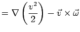
Return to viscous incompressible flow.
N-S equation:
Then,
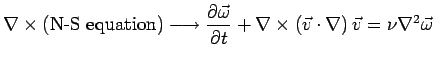
since
![]() for any
for any ![]() (conservative forces)
(conservative forces)
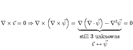
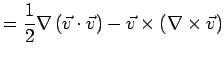
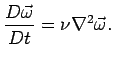
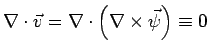
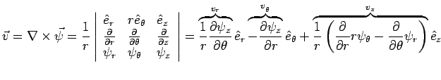
Now consider the vector identities:
 |
||
 where where |
||
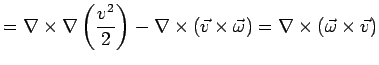 |
||
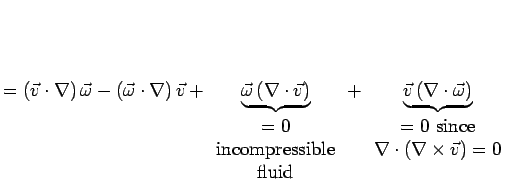 |
Therefore,
| or | ||
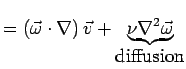 |
If
![]() then
then
![]() , so if
, so if
![]() everywhere at one time,
everywhere at one time,
![]() always.
always.
Also since ![]() 1 or 2 mm
1 or 2 mm![]() /s, in 1 second,
diffusion distance
/s, in 1 second,
diffusion distance
![]() , whereas diffusion time
, whereas diffusion time
![]() . So for a diffusion
distance of L = 1cm, the necessary diffusion time needed is
O(10)sec.
. So for a diffusion
distance of L = 1cm, the necessary diffusion time needed is
O(10)sec.
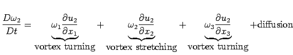
Then,
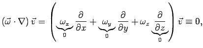
so in 2D we have
 |
If ![]() = 0,
= 0,
![]() , i.e. in 2D, following a particle, the angular velocity is conserved. Reason: in 2D, the length of a vortex tube cannot change due to continuity.
, i.e. in 2D, following a particle, the angular velocity is conserved. Reason: in 2D, the length of a vortex tube cannot change due to continuity.
 |
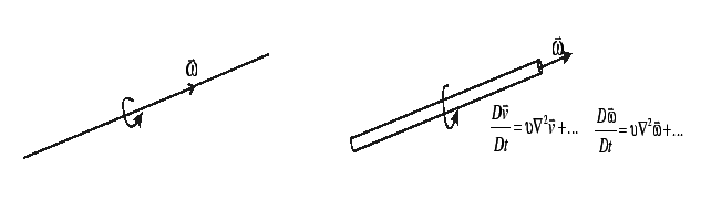
For example:

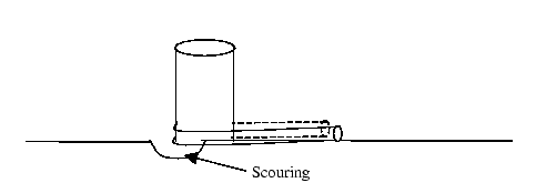
What really happens as the length of the vortex tube
L increases?
IFCF (Ideal fluid under the influence of conservative forces) is no longer a valid assumption.
Why?
Ideal flow assumption implies that the inertia forces are much larger than the viscous effects (Reynolds number).
 Length increases
 Therefore IFCF is no longer valid.
If
![]() at some time
at some time ![]() , then
, then
![]() always for ideal flow under conservative body
forces by Kelvin's theorem. Given a vector field
always for ideal flow under conservative body
forces by Kelvin's theorem. Given a vector field
![]() for which
for which
![]() , then there exists a potential function (scalar) - the velocity potential - denoted as
, then there exists a potential function (scalar) - the velocity potential - denoted as ![]() , for which
, for which
Note that
![]() for any
for any ![]() , so irrotational flow guaranteed automatically. At a point
, so irrotational flow guaranteed automatically. At a point ![]() and time
and time ![]() , the velocity vector
, the velocity vector
![]() in cartesian coordinates in terms of the potential function
in cartesian coordinates in terms of the potential function
![]() is given by
is given by

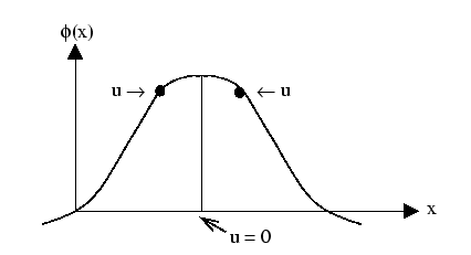
The velocity vector ![]() is the gradient of the
potential function
is the gradient of the
potential function ![]() , so it always points towards higher
values of the potential function.
, so it always points towards higher
values of the potential function.
Governing Equations:
Continuity:
Number of unknowns
![]()
Number of equations
![]()
Therefore the problem is closed. ![]() and
and ![]() (pressure) are decoupled.
(pressure) are decoupled. ![]() can be solved independently
first, and after it is obtained, the pressure
can be solved independently
first, and after it is obtained, the pressure ![]() is evaluated.
is evaluated.
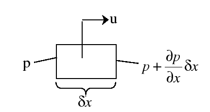
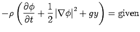
Euler eq:
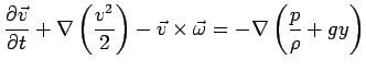 |
Substitute
![]() into the Euler's equation above, which gives:
into the Euler's equation above, which gives:
 |
or
 |
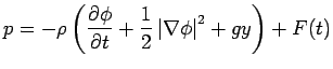
which implies that
 |
![$\displaystyle p = - \rho \left[ {\frac{\partial \phi }{\partial t} + \frac{1}{2}\left\vert
{\nabla \phi } \right\vert^2 + gy} \right] + F(t)$](img63.gif) |
Summary: Bernoulli equation for ideal flow.
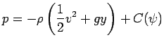 |
 |
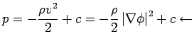 Venturi pressure (created by
velocity) Venturi pressure (created by
velocity) |
 |
 |
Note: On a free-surface
![]() .
.
Then
 for any
![]() i.e. satisfies continuity automatically.
i.e. satisfies continuity automatically.
Required for irrotationality:
For 2D flow:
![]() and
and
![]() .
.

Set
![]() and
and
![]() ,
then
,
then
![]()
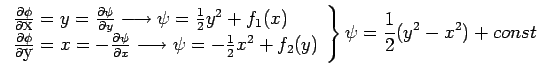
So, for 2D:
 |
Then, from the irrotationality (see (1))
![]() and
and ![]() satisfies
Laplace's equation.
satisfies
Laplace's equation.

Again let
![]() and
and
![]() , then
, then
![]() and
and
![]() .
.
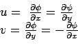
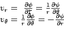
In 2D:
![]() and
and
![]() .
.
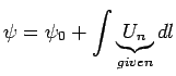
We define
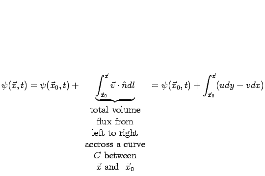 |
For ![]() to be single-valued,
to be single-valued, ![]() must be path independent.
must be path independent.
 or
or 
Therefore, ![]() is unique because of continuity.
is unique because of continuity.
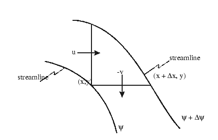
Let
![]() be two points on a given streamline
(
be two points on a given streamline
(
![]() on streamline)
on streamline)
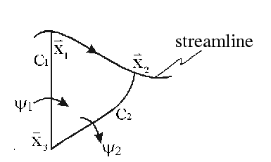
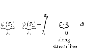 |
Therefore,
![]() ,i.e.,
,i.e., ![]() is a
constant along any streamline. For example, on an impervious
stationary body
is a
constant along any streamline. For example, on an impervious
stationary body
![]() , so
, so ![]() = constant on the body is the
appropriate boundary condition. If the body is moving
= constant on the body is the
appropriate boundary condition. If the body is moving
![]()
 on
the boddy on
the boddy |

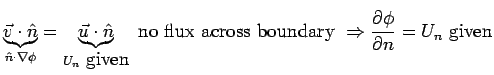
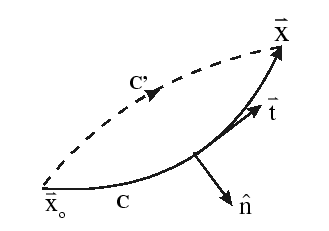
Flux
![]() .
Therefore,
.
Therefore,
![]() and
and
![]()
Summary: Potential formulation vs. Stream-function formulation for ideal flows
table
| potential | stream-function | |
| definition |
|
|
| continuity
|
|
automatically satisfied |
| irrotationality
|
automatically satisfied |
 |
| in 2D
|
|
|
| Cartesian (x, y) |
|
Cauchy-Riemann equations for ( (real, imaginary) part of an analytic complex function of z = x +iy |
| Polar (r, |
 |
| For irrotational flow | use | |
| For incompressible flow | use | |
| For both flows | use |
Given ![]() or
or ![]() for 2D flow, use Cauchy-Riemann
equations to find the other:
for 2D flow, use Cauchy-Riemann
equations to find the other:
For example: ![]() = xy
= xy ![]() = ?
= ?