 [Eq. 1]

(2) Present affiliation: Dept. d'Enginyeria Industrial, Universitat de Girona, 17071 Girona, Spain
(3) Present affiliation: Lawrence Livermore National Laboratory, Livermore, CA 94550, USA
A revised version of Report 20 was published in the Journal of Geophysical Research in 1998 (Vol. 103(D3), p. 3437-3467). A paper version of the published reprint is available by request at no cost. (Send an e-mail request; ask for REPRINT No. 98-01). Report 20 below is a slightly outdated version of that article and is missing a figure. A complete version is available in PDF format (37 kB).
Usually, the climate change and air pollution issues are studied independently, and little attention is focused on interactions and relationships between them. For example, most scientific and policy analyses of the greenhouse gas issue do not consider the likely influence of local air pollution processes and controls on global emissions, or on the cost of alternative greenhouse gas control measures. This lack of consideration of local pollution occurs in part because the climate science and policy issues are great analytical challenges by themselves; it also occurs in part because the analytical models used for assessment of the greenhouse issue cannot resolve the space and time scales of urban pollution due to computational constrains. Failure to consider the interaction between global and urban aspects of anthropogenic emissions may be a serious shortcoming in current analyses because these two aspects are linked in at least three important ways: through the chemistry of the atmosphere, through the role of combustion in each, and through the potential interaction of local pollution policies with greenhouse gas control measures.
This paper focuses on the first of these links: specifically the way in which the global and local aspects of atmospheric pollution are linked through tropospheric chemistry. For example, the chemistry that leads to urban photochemical smog (involving NOx, hydrocarbons, CO, O3 and UV light) also involves important greenhouse gases (methane and ozone). Also, aerosols resulting from SOx and NOx emissions contribute both to urban pollution and acid rain and to changes in the Earth's radiative balance.
Specifically, we have developed a parameterization or "reduced-form" model that allows us to estimate the effective emissions (EE) from an urban area as functions of the urban true emissions (E) and local meteorology (M). The relationship between EE and E is complex because the high concentrations of gases and aerosols found in polluted urban areas, combined with nonlinearities (e.g., reactions of NOx or HOx species with themselves) and interactions (e.g., reaction of NOx species with HOx species or heterogeneous reactions on aerosols), lead to different rates of production and removal when the true emissions are confined to urban areas compared with artificially spreading the same true emissions evenly over a (usually very much larger) grid cell of a global chemistry and climate model. A similar issue is addressed in a paper by Gillani and Pleim (1996). They studied the importance of sub-grid scale effects in regional models, and concluded that chemical nonlinearities lead to important differences when these effects are taken into account.
To include urban processes in a global model, we need to compute EE day-by-day for, say, the 70 urban areas of the world that will have more than 3 million inhabitants by year 2000 (WHO-UNEP, 1993). Therefore, the urban process subroutine in the global model has to be integrated over more than three million (70x365x120) days in a 120 year run of a coupled chemistry and climate model such as that of Prinn et al. (1997). This effectively prevents the direct use of any of the presently available three-dimensional urban models in a global model, and it is the impetus for the parameterization discussed here.
The CIT Urban Airshed Model (McRae et al., 1982) is the basis upon which we have built our parameterization. The CIT Urban Airshed model can deal directly with the physical and chemical phenomena that lead to the aging of pollutants within an urban domain, since the model was designed specifically to simulate these processes. This model requires hourly fields of several meteorological variables, hourly emissions of several chemical species, initial conditions and data related to the domain. A typical 1 day integration for a domain discretized in 10,000 cells requires about 1 hr of time on a fast workstation. As noted above, we cannot use directly such a model to carry out the 3 million day integrations required in the global model.
Our parameterization of the urban model uses the probabilistic collocation method (Tatang, 1994) which produces analytical expressions relating model outputs to model inputs thus enabling uncertainty analysis of computationally expensive models at a very low computational cost.
The next section (Section 2) describes the two basic components used for derivation of the parameterization: the CIT Urban Airshed Model and the collocation method. We discuss in the third section the selection of inputs and outputs and development of parameterization itself. In the fourth section, a comparison between the results obtained using the true model and the parameterization is given, followed by a sensitivity and uncertainty analysis for the parameterization. Finally, conclusions and proposals for further work are given in Section 5.
The photochemical reaction formulation employed at present in the CIT model is based on the work by Lurmann et al. (1987). This formulation is focused on fast reactions between nitrogen oxides and volatile organic compounds that drive ozone production. Transformations from NOx to nitrous and nitric acids, and from SO2 to SO3 (i.e., from oxides to aerosol precursors) are also considered. In contrast to a global model, the chemistry of longer-lived species, such as methane, is not included. Thirty-five species (single species or lumped classes) and 106 reactions are included. Sixteen of these species are treated as directly emitted species, and fourteen of them are used to set initial and boundary conditions (see Table 1). Both area and point source emissions can be handled. Hourly, grid-resolved emission data must be provided to the model. Boundary conditions, given by the combination of surface and vertical profiles of concentrations, can also have an hourly resolution if needed.
Hourly three-dimensional fields of several meteorological variables must be provided: wind, humidity, temperature, mixing layer height, and two radiation scaling factors (one for the whole solar radiation spectrum, the other for the UV light). These fields may either be derived from observed surface and sounding data or supplied by a meteorological model. The CIT Urban Airshed Model has also been coupled interactively to the United Kingdom Meteorological Office (UKMO) Mesoscale Model (Golding, 1992) to produce the Integrated Meteorological and Air Quality System (IMAQS) (Pan, 1996). For two reasons, the development of our parameterization is based on the original CIT Urban Airshed Model. First, many mesoscale meteorological phenomena are forced by the underlying topography and our desire for a computationally efficient parameterization prevented us from specifically including topography or land use. Thus, the power of the mesoscale meteorological model would not have been well utilized. Second, in order to develop the parameterization, the full model has to be run some hundreds of times and the CIT Urban Airshed Model is several times faster that the IMAQS model.
Table 1. Main species included in the CIT model.
| Main species | Directly emitted species | Initial and boundary conditions |
| CO | yes | yes |
| NO | yes | yes |
| NO2 | yes | yes |
| SO2 | yes | yes |
| O3 | yes | |
| N2O5 | ||
| HNO3 | ||
| OH | ||
| HO2 | ||
| H2 O2 | ||
| Formaldehyde | yes | yes |
| Acetaldehyde | yes | yes |
| Methyl ethyl ketone | yes | yes |
| Alkanes (C4) | yes | (a) |
| Ethene | yes | (a) |
| Alkenes (C3) | yes | (a) |
| Toluene | yes | (a) |
| Higher aromatics | yes | (a) |
| Methanol | yes | |
| Ethanol | yes | |
| NH3 | yes | |
| SO3 | yes | |
| PAN | (b) | |
| NO3 |
 [Eq. 1]
where xk is one of the K input parameters to the model f, and y is the output (or "response" to the inputs) of the model. Since there is a range of possible values for each input parameter, these inputs can be treated as random variables. Thus, the output of the model can also be considered as a random variable. The goal of the collocation method is to approximate the K-dimensional "response surface," y, by a simple polynomial function of xk. The polynomials used by the collocation technique are orthogonal polynomials Pkj (xk), defined by:
 [Eq. 2]
where gk(xk) is the probability density function (PDF) of the independent random variable xk, ij is the Kronecker delta, and C is a real number (if C=1 the polynomials are orthonormal). For example, for a gaussian PDF the Pkj are Hermite polynomials. The polynomial definition procedure is implemented using ORTHPOL (Gautschi, 1994).
Using these polynomials, the independent random variables can be written as:
 [Eq. 3]
and the dependent variable y can be approximated by a polynomial chaos expansion (PCE):
 [Eq. 4]
where y0, y i1i2...iK are coefficients to be determined, and N is the order of the approximation. By running the actual model a number of times we obtain the required number of sets of (xk, y) values to solve for y0 and all yi1i2...iK.
The orthogonal polynomials, as noted above, are used in the polynomial chaos approximation of the model. Equally important, they are also used to generate the sets of parameter values xk (the so-called collocation points) for solving for the approximation through (4) (Webster et al., 1996). Specifically, the N+1 roots of the (N+1)th order polynomial corresponding to each parameter xk are used to define the collocation points. Because these roots help define the high probability region of each input parameter, we obtain an approximation of y that is particularly good within the most probable range of values of the input parameters. Moreover, the roots of the (N+2)th order polynomials are used to define another set of collocation points which can be used to estimate the error of the approximation which, again, takes account of the actual probability distribution of the parameters. The approximation defined by (4) (which we refer to here as the "parameterization") is therefore designed to perform in the region of highest probability of the inputs. Versions of equation (4) are developed for each output variable (y) of interest.
(a) Time (DATE). The solar radiation flux driving photochemistry depends on astronomical factors (time and location) as well as atmospheric factors (reflection, absorption and scattering). The effect of time is taken into account through specifying the date in Julian days (DATE) starting with 0 on January, 1, and ending with 364 on December, 31. This input date (along with input latitude) is also used to define the mean air temperature for the site. The probability distribution for DATE is, of course, uniform (i.e., all days in the year are equally probable, Figure 1).
(b) Location (LATI). Location is specified by the latitude of the region. Although the distribution of major cities is not uniform with latitude (most of the largest cities are placed between 20 and 50 in both hemispheres), we have also for convenience defined a uniform PDF for this parameter (Figure 1). The selected range of values for this input variable (LATI) is from 0 to 67.5 degrees North and South since there are no major cities outside of this range. The parameterization which is formally derived for the Northern Hemisphere can be used for the Southern hemisphere cities simply by changing the date by 6 months. This ignores the small effect of the Earth's orbital eccentricity which presently allows more sunlight incident on the southern hemisphere than the northern hemisphere.
The longitude of the urban area is not one of the selected input parameters. The reason is that the dominant effect of longitude is the difference between local time and universal time which is accounted for by having all the runs carried out in local time.
(c) Air temperature (DTEM). Air temperature is important since rate constants for many reactions depend on temperature. Hourly fields of surface temperature are required by the CIT model. Temperature is calculated as the sum of three terms. The first is the climatic average temperature appropriate to the season and latitude of the domain which is computed using the formula proposed by North and Coakley (1979) for a symmetrized Earth:
 [Eq. 5]
Here T(,d) is the mean (in the climatic sense) temperature for latitude and day d (d=0 at December 22), T0=14.9C is the global mean temperature, T1=15.5C, T2=28.0C, and is the frequency related to the annual cycle. The root mean square error of this expression, relative to actual temperature measurements, is only 2C. The expression is convenient, since it uses two existing inputs (latitude and date) and it preserves the symmetry between hemispheres.
To take account of variability around the climatic mean, we input a parameter, DTEM, which is the difference between actual temperature and the climatic mean given by (5). The PDF corresponding to this input, is a normal distribution consistent with its definition (Figure 1).
Adding the temperature from (5) and DTEM yields a daily mean temperature. To represent the daily cycle, we assume an oscillation of 8C with the minimum at sunrise and the maximum 2 hours after noon and linear variations between these extreme values (Figure 2). While varying with time, temperatures are assumed to be uniform in space through the urban domain.
 [coming soon...]
Figure 1. Probability density functions (PDFs) for most input parameters defined in the text. The PDF for CO is the same as that for SO2, but ranges between 0 and 500 kg/km2. The PDF for DVOC is the same as for DNOX. The PDFs for all air quality indices (AQI) are the same.
Another atmospheric input required by the CIT model is hourly fields of specific humidity. Moisture content is chemically important since it plays a role in some gaseous and aqueous phase reactions, although no aqueous phase reactions are considered in the model runs discussed in this paper. In this study, we have not included specific humidity as an input parameter. Based on some previous tests, we have instead assumed relative humidity to be the same for all runs, and equal to 60%. From this relative humidity and daily average temperature, we compute the equivalent specific humidity (in g/kg). The specific humidity is then considered constant for that run, unless at the cooler night-time temperatures it would imply a relative humidity higher than 100%. Then, specific humidity is set to the saturation level. As with the other meteorological fields, the humidity field is assumed uniform in space.
(d) Cloud cover (CLOU). The CIT model requires inputs of hourly values for the scaling factors for total and ultraviolet solar fluxes. These fluxes are related to the altitude of the region and to the optical characteristics of the atmosphere. In this study we approximate the UV scaling factor by equating it to the scaling factor for total solar radiation. This latter factor can be estimated from cloud cover data using the expression proposed by McRae et al. (1992). Cloud cover in tenths of overhead sky area (CLOU) is therefore one of the chosen inputs. The derived solar total and UV radiation scaling factors are assumed constant throughout the run and uniform in space. Possible values for cloud cover range from 0 to 10 tenths. The probability distribution function assumed is uniform (see Figure 1).
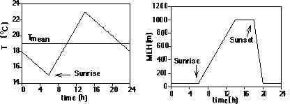
Figure 2. (a) Example of the assumed daily cycle of temperature. In this case, the mean temperature is 19C. (b) Example of the assumed daily cycle of the mixing layer height (MLH). In this example, the maximum height (i.e., the parameter MIXI) has been set to 1000 m. Note that sunrise and sunset depend on latitude and date in both cases.
(e) Mixing layer height (MIXI). Turbulence plays an important role in dispersion of an urban plume of pollutants. The CIT model parameterizes the turbulent characteristics of the atmosphere (using the turbulent diffusivities) based on solar radiation, wind, and most importantly, mixing layer height. We express the latter height in terms of the input parameter MIXI, defined as the maximum mixing layer height during the day. Mixing layer height has, like temperature, a daily cycle, which has been approximated as shown in Figure 2. At night (from two hours after sunset to sunrise), the mixing layer height is set equal to the larger of MIXI/20 or 50 m. The mixing layer height then increases linearly from sunrise to its maximum value (MIXI) two hours after noon, where it then remains until sunset. Finally, it decreases linearly to its night-time height in the two hours following sunset. Like other atmospheric fields, a uniform space distribution has been assumed. The probability distribution of MIXI is defined by a beta distribution ranging between 200 and 2000 m. The distribution (Figure 1) is asymmetrical, and the most probable value of MIXI is about 800 m.
(f) Residence time (TIME). The CIT model requires specification of the size of the urban region and the wind velocities and direction. However, given the assumed symmetry of our urban region (defined below) and uniformity of atmospheric fields, the time that pollutants reside inside the domain is the major chemically important parameter determined by the wind velocity. Hence we input the residence time, TIME, defined as the width of the urban region divided by the wind velocity, instead of the velocity separately. The probability distribution for TIME is uniform, between 6 hours and 3 days. For an area of 200 km side, that means a range of winds between 0.7 and 10 m/s.
When running the CIT model to generate the parameterization, a square region of 200 km side is assumed. It is discretized into 40x40=1600 grid cells. The urban region is assumed flat and a radially symmetric central emitting region (the city) covers almost half of the area (Figure 3). Different surface characteristics (in particular, surface roughness) have been defined for each part of the domain. The vertical structure is the same for all runs: the top is fixed at 2090 m height, and there are five layers below that with varying depth. The height of the top corresponds approximately to the maximum mixing layer heights typical of the continental environments of many large cities.
The CIT model needs hourly fields of three-dimensional winds. For development of the parameterization, information regarding wind is reduced to one single value: the mean (in space and time) wind speed in the urban area defined as the domain width (200 km) divided by TIME. The wind in any single model run is considered constant in time and uniform in space, no vertical wind is assumed, and wind direction is the same for all the runs. Although there is an expected daily variation of wind speed, related to the solar and boundary forcing and topography, it is domain specific and has not been taken into account. The assumptions of zero vertical wind and horizontally uniform wind are consistent with a flat terrain. Wind direction effects are not considered, because they have a minor contribution relative to wind speed, particularly when all the other relevant fields (terrain, emissions, boundary conditions, solar radiation, etc.) are so symmetric (Figure 3). Wind direction for all runs has arbitrarily been set perpendicular to one side of the CIT model domain.
(g) Emission of sulfur oxides (SO2). The CIT model requires hourly fields of emissions of several pollutants (see Table 1), and it can distinguish between point sources and area sources. We have assumed for all pollutants that we have area sources only distributed throughout the emitting city area in the domain. The city area is defined as a circle with a diameter 3/4 of the width of the domain. Inside this circular area, we have defined six circular bands with different emissions in each of them. The two central ones (with diameters 1/10 and 2/10 of domain width) account for 50% of total emissions. The following two (with diameters 3/10 and 4/10 of domain width) account for 25% of total emissions. The most exterior rings (with diameters 5/10 and 7.5/10 of domain width) account for the residual 25% of emissions. In terms of emissions per unit area, the ratios are 1, 0.31, 0.125, 0.075, 0.05 and 0.0125 for each circular band relative to the central part of the city (see Figure 3).
There is of course a wide range of emission patterns. For example, for coastal cities, the pattern is more linear, or, at least, does not have radial symmetry. We have checked the sensitivity of the CIT model results to different assumed patterns of emissions. Specifically, we have defined an elongated emitting region (to simulate a coastal city) and run the CIT model for this emission pattern with the city axis either perpendicular or parallel to the wind direction. The differences between these two runs and the equivalent circular city are shown in Figure 4. For some outputs, differences may reach 80%, but the average difference is around 20 % in both cases. Although these differences are noticeable, they are not larger that the errors in the derived parameterizations discussed later. Therefore, the circular city approximation is considered sufficient for our purposes.
The input parameter SO2 corresponds to the total mass of SO2 emitted per day divided by the area of the domain. Five detailed city emission inventories have been checked to define a typical range of values for this parameter (see Table 2). These values are consistent with rough estimations of emissions in several other cities of the World (WHO-UNEP, 1993). We have used a beta distribution, with limits of 0 and 50 kg/km2/day, and a maximum probability value of 10 kg/km2/day (Figure 1) to define the PDF of SO2. The value of 10 kg/km2/day corresponds to emission of 333 kg/km2/day in the most central circular band.
Although some sulfur oxides are emitted by vehicles, the main sources of this pollutant are industries, especially power plants, which generally operate on a continuous basis. Therefore, only a small amplitude daily cycle can be expected for the SO2 emissions and we therefore assume these emissions are constant in time. In addition, emission of SO3 is assumed to be 2% of the emission of SO2.
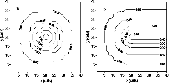
Figure 3. Examples of assumed spatial distributions of emissions and initial concentrations. a) Emissions of CO, at 12 h, in ppm m-1 min-1 (these are the units used by the CIT model to express emissions into the domain: they refer to the increase of concentration in the first computational layer, per unit of vertical length and per unit of time) when the input parameter CO is 100 kg km-2. If the domain is 200200 km2, the urban area covers a circle of 150 km diameter, and downtown (where 50% of emissions are released) occupies a circle of 40 km diameter. b) Initial concentrations of CO, in ppm, when the input parameter AQIVOC is 0.1.
(h) Emission of carbon monoxide (CO). We define the input CO as the total daily emissions of carbon monoxide divided by the domain area. The range of possible values has also been derived after investigation of several emission inventories (see Table 2). A beta distribution bounded by 0 and 500 kg/km2/day, with a most probable value of 100 kg/km2/day is used to define the PDF for this parameter (Figure 1). Emission of CO follows the same assumed spatial pattern as SO2 (Figure 3).
Carbon monoxide is mainly emitted by moving vehicles. Therefore, its emissions show a strong daily cycle that follows the pattern of the traffic cycle. Several emission inventories for developed cities (listed in Table 2) have been studied and used to define a typical daily cycle of CO. This typical cycle has high emissions between 6 a.m. and 6 p.m. and maximum emissions at 3 p.m. We realize the limitations of applying this cycle derived from developed cities to cities in developing countries, or of applying the same cycle to countries as different as the USA and Spain as far as traffic schedules are concerned. However, we believe that it is important foremost to include the fact that higher emissions occur simultaneously with higher radiation levels, and the cycle we have chosen reflects this basic correlation.
(i) Emissions of Volatile Organic Compounds (DVOC). Similar to other pollutants, emissions of several volatile organic compounds (VOC) need to be input into the CIT model on an hourly basis. Emissions of VOC have several possible sources, with road traffic being the main one in cities. Therefore, we can expect that total VOC emissions are highly correlated with CO emissions. We have verified this correlation using the emission inventories that we have available (Table 2). The linear regression relating total VOC emissions to CO emissions ECO is:
 [Eq. 6]
However, the actual amount of VOC emitted in a specific city may be different from . We therefore define the parameter DVOC, which accounts for the difference between the actual total VOC emissions, EVOC, and the emissions derived from (6):
 [Eq. 7]
For the PDF of DVOC, we have chosen a symmetric beta distribution between -0.7 and 0.7 (Figure 1).
We allocate total VOC emissions among 10 different VOC species (Table 1) using factors derived from the emission inventory for Los Angeles, USA (McRae et al., 1992) and consistent also with those derived for Melbourne, Australia (G. Adamkiewicz, unpublished data, 1996) and Mexico City (IMP-LANL, 1994). The temporal evolution and spatial pattern of VOC emissions are assumed to follow the same pattern as CO.
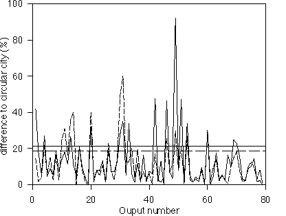
Figure 4. Differences between CIT model results when we approximate an elongated urban area by the circular area described in the text: a) solid line: the elongated domain is perpendicular to wind direction. b) dashed line: the elongated domain is parallel to wind direction. Horizontal lines show mean error for all the outputs in both cases.
Table 2. Emissions per unit area in several urban areas (kg/km2/day).
| Urban
area
|
Reference
|
CO
|
SO2
|
NOx
|
VOC
|
|---|---|---|---|---|---|
| Los Angeles | Harley et al. (1993) | 101 | 1.9 | 13.1 | 26.5 |
| Upper Rhine | Schneider et al. (1996) | 46 | 8.9 | 17.3 | 25.1 |
| Manchester | Longhurst et al. (1996) | 15 | 6.8 | 5.6 | 6.1 |
| Barcelona | Costa and Baldasano (1996) | 220 | 19.5 | 58.6 | 80.2 |
| Melbourne | Adamkiewicz (personal comm., 1996) | 138 | 2.7 | 18.7 | 36 |
| Correlation to CO emission | 0.55 | 0.89 | 0.95 |
(j) Emissions of nitrogen oxides (DNOX). The same procedure used to define VOC emissions has been applied to define emissions of nitrogen oxides because emissions of NOx, like VOC, are highly correlated with emissions of CO (Table 2). The NOx emissions () derived from ECO using linear regression are:
 [Eq. 8]
As for VOC, a parameter, DNOX, is defined to take account of differences between actual emissions and . DNOX has the same PDF as DVOC. Ninety-five percent of NOx emission (by mass) is assumed to be NO, while the other 5% is assumed to be NO2. NOx emissions follow the same spatial and temporal distributions as CO and VOC.
Sillman et al. (1990) noted that the emission ratio r=EVOC/ENOx may be used to distinguish typical urban emissions from point sources (e.g., power plants). When r is computed as atoms of C over atoms of N by volume, r < 1 for power plants; and r > 1 for urban areas (where typically r 5). Using the above correlations between NOx, VOC, and CO emissions, r 4. By setting the parameters DNOX and DVOC at their minimum and maximum values we see 1 < r < 9.
(k) Initial and boundary conditions (AQINOX, AQISO2, AQIVOC, AQIOZO). The mass of pollutants both present inside the domain when the simulation starts and entering the domain through the boundaries are very important for the photochemistry. To simplify the amount of input data required, we simply express the initial and boundary condition information using four so-called Air Quality Indexes (AQI). These AQI, denoted AQINOX, AQISO2, AQIVOC, and AQIOZO determine initial concentrations and boundary concentrations for NO and NO2, SO2, VOC and CO, and ozone and PAN respectively. These AQI vary from 0 to 1 and represent fractions of maximum concentrations for each species or group of species. The maximum concentrations are appropriate for polluted atmospheres as given in Seinfeld (1986), Finlaysonn-Pitts and Pitts (1986), and the U.S. NAAQS and other standards (see Table 3). Runs begin and initial conditions apply at midnight. To estimate maximum concentrations for formaldehyde, acetaldehyde, methyl ethyl ketone and other VOC from the total concentration of reactive hydrocarbons, RHC, we have slightly modified the factors provided in the CIT User's Manual (McRae et al., 1992). We assume a beta distribution between 0 and 1 for the PDF of each AQI (Figure 1). The most probable value is assumed to be 0.1, which corresponds to a quite clean atmosphere. The justification for the latter assumption is that boundary conditions are set through these AQI values, and we assume that the non-urban area around the city is not usually very polluted.
Table 3. Concentrations for defining AQI (see text) (in ppb by mole).
| Pollutant |
Clean troposphere(a) |
Polluted troposphere(a) |
WHO Air Quality Guideline |
NAAQS |
Value for AQI=1 |
| CO | 200-1000 | 1000-50000 | 25000 (1 h) (b) | 35000 (1 h) | 4000 |
| SO2 | 1-10 | 20-200 | 125 (1 h) | 500 (3 h) | 100 |
| NO2 | 0.1-20 | 50-500 | 190 (1 h) | 50 (annual) | 300 |
| NO | 0.01-20 | 50-2000 | 500 (1 h) | 100 | |
| RHC(c) | 100-500 | 500-1500 | 240 (3 h) | 1000(d) | |
| O3 | 20-80 | 100-500 | 100 (1 h) | 120 (1 h) | 250 |
Initial concentrations vary throughout the domain. The values given by multiplying the maximum concentrations by the AQI are assumed to apply to city center and downwind from it (Figure 3). At different distances from the center, initial concentrations are assumed to be lower, so that at the upwind boundary, the concentration is 0.1 times the central concentration (see Figure 3). Boundary conditions are kept constant for the whole run.
 [Eq. 9]
where Mi(t) is the total mass of species i in the domain after t hours; Mi(0) is the mass at the beginning of the run (initial conditions); Fi in(0,t) and Fiout(0,t) are respectively the total amounts of species i that have entered and exited the domain through the boundaries, over time t; Ei(0,t) is the true emission of species i over time t; and Ri(0,t) is the amount of species added (positive) or removed (negative) in the domain by chemical reactions between t=0 and t. The effective emission (EEi(t)), is defined as the sum of the true emissions and the net production or destruction due to chemistry. Since the CIT model does not provide explicitly the term Ri, we derive the effective emissions using:
 [Eq. 10]
Since the long-term average of Mi(t)-Mi(0) (accumulation in domain) is generally much less than the long-term average for Finet(t)=Fiout(0,t)-Fiin(0,t) (net export from domain) then, over the long term, the effective emissions equal approximately the export of pollutants from the domain. EEi may be aged primary emissions or production of secondary pollutants, depending upon the species. In principle, EEi, like Ri, may have positive or negative values.
We are interested in the effective emissions of (primary) species that are actually emitted (NO, NO2, CO, SO2, SO3 and some VOC species) and (secondary) species generated by chemistry (O3, HNO2, HNO3, HNO4 and PAN).
We typically run the CIT model for one day. This length of time is of the same order than the mean residence time of pollutants in the domain and enables resolution of the effects of the daily cycles of emissions and solar radiation. We could output the effective emissions every hour; to reduce the number of outputs, but still define the daily cycle, we output results every six hours.
In summary, the outputs that we include in our parameterization are: the total mass inside the domain at the beginning of the simulation, and after 6, 12, 18 and 24 h (Mi(0), Mi(6), Mi(12), Mi(18), Mi(24)) and the net export fluxes after 6, 12, 18 and 24 h (Finet(0,6), Finet(0,12), Finet(0,18), Finet(0,24)) for all species. All these outputs are expressed per unit area. In addition, we output quantities that are useful air pollution indicators: domain-averaged and 8 h-averaged concentrations for some pollutants (SO2, NOx, CO and O3), total SO2 deposition every 8 hours, and maximum ozone concentration and the time when the peak is reached. These latter outputs allow us the use of the parameterization in assessment of local air pollution control policies.
Since we are potentially interested in 31 species, and nine outputs for every species, plus the 17 additional air pollution-related outputs, we have a total of 296 outputs, and hence need to generate 296 parameterizations. This is not computationally demanding, since the same number of runs of the CIT model is needed for one output as for multiple outputs. The required number of runs of the CIT model is instead defined by the number of inputs and the desired level of accuracy of the approximation. For example, to obtain the 296 parameterizations with 14 inputs, the first order (N=1) approximation requires 15 runs, the second order (N=2) approximation requires 120 runs, and the third order (N=3) needs 680 runs. The rapid increase in the number of runs needed with increasing order of the approximation is due to the increasing number of possible cross products which can involve up to 14 polynomials of the input parameters (see equation (4)).
We can in addition take advantage of any a priori knowledge about the CIT model response surface to improve the approximation. In particular, we know that the response surface is periodic regarding the parameter DATE. Since a second order polynomial expression does not have a periodic behavior, we augment the expansion by including a cosine function. The parameterization that we derive is, specifically, a second order polynomial expansion for 13 input variables (all except DATE) multiplied by a function of the input DATE that takes account of the annual cycles in output y:
 [Eq. 11]
 [Eq. 12]
Here x1 is the input DATE, x2,...,x14 are the other 13 inputs, A and XX?XX are the amplitude and the phase angle to be found for each set of input parameters, and y0 is the mean value for the output.
Based on physical reasoning, there are specific constrains on outputs: Mi(t) 0; Finet(t) -Fiin(t); deposition and concentration 0; and the time of peak ozone concentrations lies in the range 0 to 24 h. Due to space limitations, the large number of coefficients that multiply each polynomial to define each output, and the orthogonal polynomials corresponding to each input are not given here. Instead, Fortran and C versions of the parameterizations are available by contacting the authors.
Table 4. Index of agreement, d, for all the outputs
| Species | M(0) | M(6) | Fnet(0-6) | M(12) | Fnet(0-12) | M(18) | Fnet(0-18) | M(24) | Fnet(0-24) |
| NO | 0.9997 | 0.9522 | 0.7372 | 0.9134 | 0.9256 | 0.8655 | 0.9379 | 0.7732 | 0.8944 |
| NO2 | 0.9999 | 0.9594 | 0.9579 | 0.9641 | 0.9506 | 0.8925 | 0.9392 | 0.891 | 0.9315 |
| O3 | 0.9999 | 0.9786 | 0.9352 | 0.8488 | 0.942 | 0.9491 | 0.9116 | 0.9505 | 0.8979 |
| HNO3 | 1 | 0.9084 | 0.9395 | 0.9381 | 0.9408 | 0.9468 | 0.9464 | 0.9357 | 0.9389 |
| CO | 0.9982 | 0.9884 | 0.9224 | 0.984 | 0.9503 | 0.9868 | 0.9726 | 0.9863 | 0.9829 |
| HCHO | 0.9982 | 0.9906 | 0.9297 | 0.9518 | 0.9451 | 0.9718 | 0.9347 | 0.9798 | 0.9519 |
| ALD2 | 0.9975 | 0.9871 | 0.9471 | 0.9662 | 0.953 | 0.9464 | 0.9417 | 0.947 | 0.9545 |
| MEK | 0.9946 | 0.9829 | 0.9269 | 0.9764 | 0.9492 | 0.9813 | 0.951 | 0.9819 | 0.9634 |
| PAN | 0.9999 | 0.9775 | 0.9483 | 0.9171 | 0.9149 | 0.9018 | 0.8351 | 0.8925 | 0.8527 |
| ALKA | 0.9993 | 0.9909 | 0.9341 | 0.9777 | 0.9565 | 0.9606 | 0.9546 | 0.9703 | 0.9645 |
| ETHE | 0.9993 | 0.9911 | 0.9322 | 0.9566 | 0.9507 | 0.9159 | 0.9322 | 0.9452 | 0.9366 |
| ALKE | 0.9993 | 0.9521 | 0.8928 | 0.6943 | 0.8787 | 0.6032 | 0.8004 | 0.7408 | 0.7819 |
| TOLU | 0.9993 | 0.9909 | 0.9341 | 0.9697 | 0.9564 | 0.9445 | 0.9484 | 0.9635 | 0.9544 |
| AROM | 0.9993 | 0.9904 | 0.9249 | 0.7244 | 0.9253 | 0.6787 | 0.829 | 0.8417 | 0.799 |
| SO2 | 0.9994 | 0.9909 | 0.9465 | 0.985 | 0.9601 | 0.9784 | 0.9757 | 0.9859 | 0.9859 |
| SO3 | 1 | 0.991 | 0.6395 | 0.9526 | 0.9362 | 0.9375 | 0.9351 | 0.9486 | 0.9438 |
| 0-8 h | 9-16 h | 17-24 h | |||||||
| SO2 dep. | 0.8829 | 0.9291 | 0.8851 | ||||||
| SO2 conc | 0.8916 | 0.923 | 0.8612 | ||||||
| CO conc | 0.9462 | 0.9521 | 0.8508 | ||||||
| NOx conc | 0.9046 | 0.9085 | 0.7465 | ||||||
| O3 conc | 0.8921 | 0.9337 | 0.8855 | ||||||
| O3 peak | 0.8226 | O3 time | 0.5658 |
Wilmott (1982) has suggested that several statistical indexes, such as the mean bias error, the root mean square error, the mean absolute error, the intercept and the slope of the least-squares regression, among others, should be reported when analyzing a model's performance. As a summary of all these measures, he proposed an "index of agreement" d defined by:
 [Eq. 13]
where the subscript T denotes true model results, the subscript A denotes parameterization results, and the over bar denotes the mean value. P (=100) is the number of comparisons used to check the error. With this definition, the better the model, the closer d is to unity. Wilmott (1982) notes that this index, which is both relative and bounded, is particularly useful for comparing different models with the same set of inputs and outputs. In our case, we use it to compare the second order parameterizations to the parent CIT model.
The values for d for each output are shown in Table 4. Most d values are evidently close to unity indicating the parameterization is a quite good approximation for most of the outputs. Only for a very few outputs is the index of agreement below 0.75. Specifically, the time when the peak ozone concentration is reached is poorly approximated (d = 0.5658). This result could be expected, since the second order expansion does not provide high time resolution and the time when peak ozone occurs is a non-linear function of the input parameters.
Correlations between parameterization and CIT model outputs are generally good (Figure 5). The points in Figure 5 that are far from the perfect correlation lines generally correspond to a set of input values that is very unlikely to happen (i.e., one or more input parameters take a value close to the limit of their PDFs, represented in the figure by open squares). Again the only exception to the goodness of the parameterizations is the time for peak ozone concentration. Except for this time, linear regressions between CIT model and parameterization show intercept values close to 0, slopes close to 1, and correlation coefficients exceeding 0.6.
To determine PDFs for each output, we have run the 296 parameterizations 10,000 times with sets of input parameters generated by Monte Carlo sampling within the ranges defined for each. Results for the total net flux of 9 species through lateral boundaries in one day (Finet(0,24)), sulfur dioxide deposition, peak ozone concentration and the time when this peak is reached are shown in Figure 6. Note that net fluxes are usually biased towards positive values indicating that the flux of pollutants leaving the urban region exceeds the flux of pollutants entering, asexpected. For some species (e.g., ozone) the net flux can be negative indicating efficient net destruction rather than production of these species in certain circumstances. The SO2 deposition flux may reach 0.1 kg/km2 per day, although in general it is less than 0.03 kg/km2. Similarly, the peak ozone concentration may reach 0.1 ppm, but usually it is well below 0.06 ppm. Although this value may seem low, note that we define the peak to be the maximum domain averaged concentration. The actual peak in a specific grid cell in the domain may be two to five times higher than the domain average. Consistently with previously noted results, the PDF for the time of peak ozone does not have any significant pattern.
We have carried out two types of sensitivity analyses. First, DEMMUCOM provides the contribution of each input parameter to the variance of the outputs (Table 5). Note that the residence time, as well as certain air quality indices and emissions are the inputs that explain most of the variance for most of the outputs. Specifically, residence time is the most important contributor to the variance of half of the analyzed outputs. This makes sense, since the residence time is the parameter that defines how long pollutants undergo chemical reactions in the domain. The input CO is also very important since this parameter also determines emissions of NOx and VOC through the correlations (6) and (8). The air quality indexes for NOx, VOC, and ozone, which determine initial and boundary conditions in the simulation, are also important parameters. Note that while the SO2 emissions and SOx air quality index appear less important, this is misleading because the number of outputs related to SOx is much less than the number of outputs related to NOx-VOC-O3 photochemistry. The parameter LATI is quite important, since it drives (along with DATE) the incoming solar radiation and the temperature. Note that DATE does not appear in this analysis, since, as explained earlier, the seasonal effect has been considered external to the collocation method. Among meteorological inputs, the mixing layer height (MIXI) is the most important, especially for concentration related outputs. MIXI is naturally not important for outputs of the total amount of pollutants in the domain (as opposed to concentration), and it also has no effect at night when MIXI/20 is less than 50 m (its default minimum). The deviation from climatic temperature (DTEM) and cloudiness (CLOU) have in general a minor contribution to the variance of the analyzed outputs. For CLOU, this result is related simply to the fact that approximately half of the outputs correspond to nighttime (at 6 h and at 24 h) when cloud effects are not relevant.
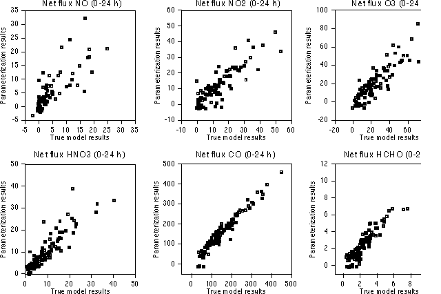
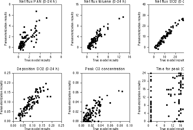
Figure 5. Sample of comparisons between parameterization results and true model results. We have chosen 12 out of the 296 outputs. Here, a total of 100 runs using sets of input parameters generated randomly are shown. Full squares correspond to points whose input parameters lie inside the range of sampling values used to generate the approximation. Open squares have one or more parameters outside that range.
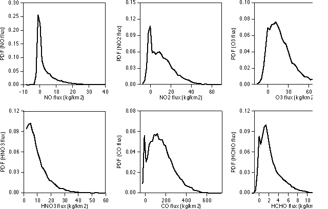
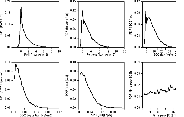
Figure 6. Probability density functions for selected outputs obtained by running the parameterizations 10,000 times with different sets of Monte Carlo generated input parameters.
Our second sensitivity analysis addresses the behavior of one output when changing one or more inputs. Since we have chosen 14 input parameters, each parameterization has a 14-D response surface. Obviously, we cannot easily represent a 14-D surface, but we can show 1-D or 2-D sections through this hypersurface. For two outputs (total mass of ozone after one day and net export flux of ozone during one day), several 1-D sections are shown in Figure 7. They have been obtained by following this procedure. First, a set of reference values for the input parameters was chosen (DATE=182, LATI=40 oN, DTEM=0, CLOU=5, MIXI=1000 m, TIME = 129600 s, SO2=10 kg/km2/day, CO=100 kg/km2/day, DNOX=0, DVOC=0, AQINOX=0.1, AQISOX=0.1, AQIVOC=0.1, AQIOZO=0.1). These reference values are the most probable values for non-uniform distributions, and central values for uniform distributions. Then, we allowed one input parameter at a time to vary between its limits, keeping all other parameters constant. The sensitivity of O3 related outputs to the inputs SO2 and AQISO2 is not shown, since this sensitivity is negligible.
Table 5. Input parameters sorted by their contribution to the variance of the outputs
| Input |
Explains most of the variance for this number of outputs |
|
| TIME | 67 | 0 |
| AQIVOC | 18 | 0 |
| CO | 23 | 3 |
| AQINOX | 11 | 0 |
| LATI | 2 | 0 |
| AQIOZO | 7 | 2 |
| MIXI | 5 | 4 |
| NOX | 2 | 3 |
| CLOU | 0 | 7 |
| TEMP | 0 | 4 |
| VOC | 1 | 16 |
| AQISOX | 4 | 30 |
| SO2 | 5 | 76 |
Total mass and net flux of ozone are both larger for DATE values around 200 (summer at 40 o N) when both solar irradiance and temperature are higher. Highest ozone mass and net flux occur in the tropics (LATI close to 0), which is reasonable since these latitudes receive maximum of solar radiation. The ozone mass and flux increase with increasing temperatures (DTEM) due to the dependence of key reactions rates on temperature. The effect of cloud increases is, as expected, to lower ozone generation. The deeper the mixing layer, the larger the ozone total mass and net flux. Deeper mixing layers mean the same amount of emissions enter a larger air mass, which, due to chemical nonlinearity, leads to enhanced ozone generation. The longer the residence time, the larger the mass accumulated in the domain and the lower the net flux of ozone. Conversely, for short residence times, ozone generation is small and ozone is advected rapidly out of the domain. The sensitivity of ozone to the parameter CO is apparently small. Recall that CO refers not only to carbon monoxide emissions, but it also defines emissions of NOx and VOC. The highest accumulation of O3 is reached with low CO (i.e., low CO, NOx and VOC emissions) but we caution that the approximation in the limit of very high emissions may be poor, since the beta function PDF of CO has small probability in that limit. The effect of the input parameters DNOX and DVOC (i.e., differences of the emissions of NOx and VOC from those defined by CO) is also shown in Figure 7. The amount of ozone created is lower when the emissions of NOx relative to CO are higher. On the other hand, the amount of ozone generated increases when the emissions of VOC, relative to CO, increase. In summary, the higher the ratio of VOC to NOx emissions, the higher the generation of ozone. Recall that this result is for a given reference set of the other input parameters. Finally, the effect of the indexes AQI (which determine both initial and boundary conditions) is also very important. The results for AQINOX show that higher ozone creation occurs with either clean or polluted NOx atmospheres. In contrast, the generation of ozone is lower in clean VOC atmospheres. The effect of increasing AQIOZO is, of course, to add more ozone at the beginning of the simulation. This results in more ozone at the end, and also in a larger flux through the boundaries.
A major proposed application of the parameterization developed here is to estimate effective emissions of pollutants from large urban areas using equation (10) in global scale chemical models. Hence this parameterization has been derived in such a way that it can be run sequentially at 6, 12, or 24 hours time steps for each polluted urban region in the global model. The relevant parameterization outputs are the net fluxes through the boundaries during the 6-24 hour run, and the total masses of pollutants in the urban domain after each run. The masses at the end of one run are then used to set the initial conditions for the next run. However, some corrections must be made. First, at the end of one run, we find amounts of pollutants present in the upper layers, depending on the maximum extent of the mixing layer during that run. However, the initial conditions for the next run assume that the two upper layers contain no pollutants. Therefore, some of the mass present inside the domain at the end of one run is not going to be present at the beginning of the next run, and must be accounted for as an extra (upper ventilation) flux of pollutants from the urban area into the global model. Second, initial concentrations of several pollutants are set through the same air quality index (e.g., NO and NO2 through AQINOX). This means that initial concentrations always show the same relative amounts of such pollutants (in the case of NOx, the ratio is 1 ppm of NO for 3 ppm of NO2). This initial ratio, of course, changes during the run due to the urban emissions and chemistry. Again, for some pollutants some mass has to be removed from the urban domain, and accounted for as another extra (AQI inconsistency) flux into the global model. In Figure 8 upper ventilation and AQI inconsistency fluxes for some specific cases are shown. Note that the upper ventilation flux depends strongly on mixing layer height, while the AQI inconsistency flux varies widely depending on the species. The effective emissions to be used by the global model are, therefore, the sum of three fluxes: the net flux through the boundaries (given as one of the parameterization outputs), the upper ventilation flux, and the AQI inconsistency flux. In this way, we ensure mass conservation for all species.
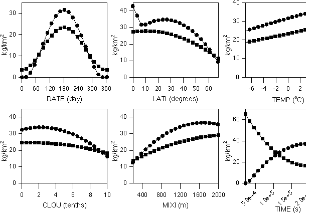
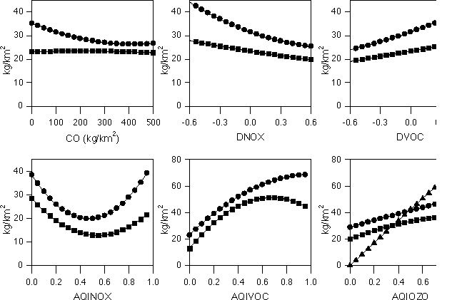
Figure 7. Sensitivity of the total mass of ozone in the domain after one day (circles) and net flux through the lateral boundaries during one day (squares) to variations in the indicated inputs. In the bottom right hand plot, the triangles refer to the initial mass in the domain.
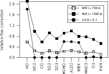
Figure 8. Examples of fluxes to be added to lateral fluxes due to upper ventilation (squares) and AQI inconsistency (circles) (see text). Fluxes are added to ensure mass conservation. Here, they are plotted as values relative to the corresponding net lateral fluxes.
The principal result of our work is the definition of a set of polynomial expressions that approximate the predictions by the CIT Urban Airshed Model for effective emissions of several species, as functions of fourteen input parameters. Specifically,
 [Eq. 14]
where effective emissions of species i at time t (EEit) are a function of actual emissions of several species (Ej) and of other urban domain properties (M) such as meteorology. The total mass inside the urban domain and the net fluxes out of the domain of NO, NO2, HNO2, HNO3, HNO4, O3, CO, PAN, SO2, SO3, and several VOC species, among other species, after 6, 12, 18 and 24 h of photochemical activity are estimated. The domain averaged and time averaged concentrations of SO2, NOx, CO, and O3, and the total deposition of SO2 are also estimated through other parameterizations. All these parameterizations need fourteen input values: the latitude of the city, the date of the simulation, the temperature, cloud cover and mixing layer depth (one value for each meteorological parameter), the estimated residence time (defined as the ratio between length of domain and mean wind), the emissions of CO, NOx, VOC and SO2, and finally four air quality indexes describing the initial pollution in the urban area of interest and the environment surrounding this area.
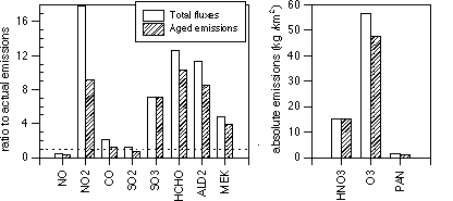
Figure 9. Examples of total fluxes out of an urban domain into a global scale model for several species. Left, for primary species, fluxes are shown relative to their corresponding actual (surface) emissions. Right, for secondary species, absolute values are given.
To develop the parameterization we applied the probabilistic collocation method, which uses the probability density functions of the inputs to generate a set of orthogonal polynomials which form the basis for a polynomial chaos expansion that approximates the actual response of the CIT model to its inputs. To simulate the seasonal cycle the polynomial expansion is augmented by a cosine function. The parameterization provides a computationally very efficient simulation of the behavior of the actual model. By comparing the outputs of the parameterizations with the outputs of the true model, we conclude, in general, that the second order polynomial expansion is adequate for our purposes.
One use of these parameterizations is to facilitate inclusion of urban-scale processes as sub-grid scale phenomena in global-scale models. Corrections to the parameterizations to ensure mass conservation in this application are given. Another use, demonstrated in this paper, is for uncertainty and sensitivity analyses. Both of these uses are based on the capability of carrying out hundreds or thousands of runs of the parameterizations in a very short time.
Certain improvements and extensions are suggested for the future based on this work. First, the probabilistic collocation methodology could be used to obtain separate parameterizations for different types of large cities (defined by their shape, location, topography, etc.). Alternatively, a set of parameterizations could be used as a basis to simulate any specific city as a linear combination of the members of the set. Second, a detailed study of the quality of the approximations, involving not only comparisons with true model results but also with observations, is needed. For this purpose, there are some cities for which detailed emission inventories and meteorological and air quality data are available. Third, a more detailed sensitivity analysis for all the outputs that we have parameterized (including simultaneous changes in two or more inputs) is desirable and will be the object of a later paper. Fourth, the implementation of the parameterizations in global chemistry models is of course the ultimate goal. The use of this parameterization in the MIT global chemistry and climate model (Prinn et al., 1997) is underway, and will also be addressed in a future report. Finally, the use of this parameterization as a fast tool for real-time urban air pollution control is also possible.
Calbó, J., W. Pan, M. Webster, R.G. Prinn and G.J. McRae, Parameterization of urban-scale photochemistry in global chemistry models (abstract), Eos Transactions, AGU, 77(46), F84, 1996.
Costa, M. and J.M. Baldasano, Development of a source emission model for atmospheric pollutants in the Barcelona area, Atmospheric Environment, 30(2), 309-318, 1996.
Finlayson-Pitts, B.J. and J.N. Pitts, Atmospheric Chemistry: Fundamentals and Experimental Techniques, 1098 pp., John Wiley and Sons, New York, 1986.
Gautschi, W., Algorithm 726: ORTHPOL - A package of routines for generating orthogonal polynomials and Gauss-type quadrature rules, ACM Transactions on Mathematical Software, 20(1), 21-62, 1994.
Gillani, N.V. and J.E. Pleim, Sub-grid scale features of anthropogenic emissions of NOx and VOC in the context of regional Eulerian models, Atmospheric Environment, 30(12), 2043-2059, 1996.
Golding, B.W., An efficient non-hydrostatic forecast model. Meteorology and Atmospheric Physics, 50, 89-103, 1992.
Harley, R.A., A.G. Russell, G.J. McRae, G.R. Cass, and J.H. Seinfeld, Photochemical Modeling of the Southern California Air Quality Study. Environmental Science and Technology, 27, 376-388, 1993.
IMP-LANL, Mexico City Air Quality Research Initiative. Volume III: Modeling and Simulation, Report LA-12699, UC-902, 122 pp., Instituto Mexicano del Petroleo and Los Alamos National Laboratory. Available through the U.S. NTIS and at the Los Alamos N.L. website, 1994.
Longhurst, J.W.S., S.J. Lindley, D.E. Conlan, D.J. Rayfield and T. Hewison, Air quality in historical perspective: a case study of the Greater Manchester conurbation, in Urban Air Pollution, Vol. 2, edited by H. Power and N. Moussiopoulos, pp. 69-109, Computational Mechanics Publications, Southampton, UK, 1996.
Lurmann, F.W., W.P Carter and L.A. Coyner, A surrogate species chemical reaction Mechanism for urban-scale air quality simulation models, Volume 1- Adaptation of the mechanism, Final report to the U.S. EPA under contract No. 68-02-4104, ERT Inc. and Statewide Air Pollution Research Center, University of California, 1987.
McRae, G.J., W.R. Goodin and J.H. Seinfeld, Development of a Second Generation Mathematical Model for Urban Air Pollution: I. Model Formulation, Atmospheric Environment, 16, 679-696, 1982.
McRae, G.J., A.G. Russell and R.A. Harley, CIT Photochemical Airshed Model: Data Preparation Manual, 127 pp., Carnegie Mellon University and California Institute of Technology, 1992.
Milford, J.B., A.G. Russell and G.J. McRae, A New Approach to Photochemical Pollution Control: Implications of Spatial Patterns in Pollutant Responses to Reductions in Nitrogen Oxides and Reactive Organic Gases, Environmental Science and Technology, 23(10), 1290-1301, 1989.
North, G.R. and J.A. Coakley, Jr., Differences between Seasonal and Mean Annual Energy Balance Model Calculations of Climate and Climate Sensitivity, Journal of Atmospheric Sciences, 36, 1189-1204, 1979.
Pan, W., The Role of Aerosols in the Troposphere: Radiative Forcing, Model Response, and Uncertainty Analysis, Ph.D. thesis, Report 43, Center for Global Change Science, Massachusetts Institute of Technology, Cambridge, Ma., 259 pp., 1996.
Prinn, R., H. Jacoby, A. Sokolov, C. Wang, X. Xiao, Z. Yang, R. Eckaus, P. Stone, D. Ellerman, J. Melillo, J. Fitzmaurice, D. Kicklighter, G. Holian and Y. Liu, Integrated Global System Model for Climate Policy Assessment: Feedbacks and Sensitivity Studies, Climatic Change, submitted, 1997.
Schneider, Ch., Ch. Kessler and N. Moussiopoulos, Influence of emission input data on ozone level predictions for the Upper Rhine valley, in Urban Air Pollution, Vol. 2, edited by H. Power and N. Moussiopoulos, pp. 1-39, Computational Mechanics Publications, Southampton, UK, 1996.
Seinfeld, J.H., Atmospheric Chemistry and Physics of Air Pollution, 731 pp., John Wiley and Sons, New York, 1986.
Sillman S., J.A. Logan and S.C. Wofsy, A regional scale model for ozone in the United States with subgrid representation of urban and power plant plumes, Journal of Geophysical Research, 95(D5), 5731-5748, 1990.
Tatang, M.A., Direct Incorporation of Uncertainty in Chemical and Environmental Engineering Systems, Ph.D. thesis, Massachusetts Institute of Technology, Cambridge, Ma., 1994.
Tatang, M.A., W. Pan, R.G. Prinn and G.J. McRae, An efficient method for parametric uncertainty analysis of numerical geophysical models, Journal of Geophysical Research, in press, 1997.
Webster, M., M.A. Tatang and G.J. McRae, Application of the Probabilistic Collocation Method for an Uncertainty Analysis of a simple Ocean Model, Report No. 4, 21 pp., MIT Joint Program on the Science and Policy of Global Change, Cambridge, Ma., 1996.
WHO-UNEP, Urban Air Pollution in Megacities of the World, 230 pp., World Health Organization - United Nations Environment Program, Oxford Blackwell Publishers, Oxford, UK, 1993.
Wilmott, C.J., Some Comments on the Evaluation of Model Performance, Bulletin American Meteorological Society, 63(11), 1309-1313, 1982.
| Top of page |