
May 1998
A revised version of
Contents
Global climate change is the subject of policy debate within most nations, and of negotiations within the Conference of Parties (COP) to the Framework Convention on Climate Change (FCCC). To inform the processes of policy development and implementation, there is need for integration of the diverse human and natural components of the problem. Climate research needs to focus on predictions of key variables such as rainfall, ecosystem productivity, and sea-level that can be linked to estimates of economic, social, and environmental effects of possible climate change. Projections of emissions of greenhouse gases and atmospheric aerosol precursors need to be related to the economic, technological, and political forces, and to the expected results of international agreements. Also, these assessments of possible societal and ecosystem impacts, and analyses of mitigation strategies, need to be based on realistic representations of the uncertainties of climate science.
Toward the goal of informing the policy process, we have developed an Integrated Global System Model (IGSM) consisting of a set of coupled sub-models of economic development and associated emissions, natural biogeochemical cycles, climate, and natural ecosystems. In this paper we describe the framework of the model and show the results of sample first runs and a sensitivity analysis.
The IGSM attempts to include each of the major areas in the natural and social sciences that are relevant to the issue of climate change. Furthermore, it is designed to illuminate key issues linking science to policy. For example, how do the uncertainties in key component models, like those for ocean circulation and atmospheric convection, affect predictions important in policy analysis? Are feedbacks between component models, such as climate-induced changes in oceanic and terrestrial uptake of carbon dioxide, atmospheric chemistry, and terrestrial emissions of methane, important for making policy decisions? To answer such questions, and allow examination of a wide variety of proposed policies, the global system model must address the major human and natural processes involved in climate change, (Schneider, 1992; Prinn and Hartley, 1992; IPCC, 1996a) and also be computationally feasible for use in multiple 100-year predictions.
The issue of computational feasibility is crucial. Priorities must be set as to what is important and what is not important in the construction. We could simply couple together the most comprehensive existing versions of the component models. However, the resulting apparatus would be computationally so demanding that the many runs needed to understand inter-model feedbacks, address a wide range of policy measures, and study uncertainty would not be feasible with any current computer. Thus a major challenge in development of the global system model is to determine what processes really need to be included in detail, and which can be omitted or simplified.
The framework of the IGSM is shown schematically in Figure 1. Human activity leads to emissions of chemically and radiatively important trace gases. The anthropogenic emissions model incorporates the relevant demographic, economic, and technical forces involved in this process. Natural emissions of trace gases must also be predicted, and for this purpose the natural emissions model takes account of changes in both climate and ecosystem states.

Finally, as shown in Figure 1, the coupled chemistry/climate model outputs drive a terrestrial ecosystems model. This model then predicts vegetation changes, land carbon dioxide (CO2) fluxes, and soil composition which can feed back to the climate model, chemistry model, and natural emissions model. Not included in the present model, but planned for future versions, are the effects of changes in land cover and surface albedo on climate, and the effects of changes in climate and ecosystems on agriculture and anthropogenic emissions.
The IGSM has several capabilities which are either not present or are simplified in other integrated models of the global climate system. Differences between our model and others were summarized by the IPCC (1996b, Ch. 10). The prediction of global anthropogenic emissions is based on a regionally disaggregated model of global economic growth. This allows treatment of a shifting geographical distribution of emissions over time and changing mixes of emissions, both of which affect atmospheric chemistry. Also, our model of natural emissions is driven by, and in later versions will be coupled to, the models for climate and land ecosystems which provide the needed explicit predictions of temperature, rainfall, and soil organic carbon concentrations.
Another special aspect of our approach is use of a longitudinally averaged statistical-dynamical climate model which is two-dimensional (2D) but which also resolves the land and ocean (LO) at each latitude (and so is referred to as the 2D-LO model in the discussion to follow). It includes a simplified ocean model which is coupled to the atmosphere and includes representations of horizontal heat transport in the uppermost ("mixed") layer and heat exchange between the mixed layer and deep ocean. It is capable of reproducing many characteristics of the current zonally-averaged climate, and its behavior and predictions are similar to those of coupled atmosphere-ocean three-dimensional general circulation models (GCMs), particularly the NASA Goddard Institute for Space Studies (GISS) GCM from which it is derived. The 2D-LO model is about 20 times faster than the GISS GCM with similar latitudinal and vertical resolution. By choosing this climate model, we are able to incorporate detailed atmospheric and oceanic chemistry interactively with climate with sufficient detail to allow study of key scientific and policy issues.
The IGSM chemistry-climate treatment is in contrast to other assessment model frameworks which incorporate highly-parameterized models of the climate system that do not explicitly predict circulation, precipitation or detailed atmospheric chemistry, such as the MAGICC model (Wigley and Raper, 1993; Hulme, Raper, and Wigley, 1995), the AIM model (Matsuoka et al., 1995), and the IMAGE 2 model (de Hann et al., 1994). These simplified models of climatic response to greenhouse gases also explicitly predict only annually-averaged global mean (e.g., AIM, MAGICC) or zonal mean (e.g., IMAGE 2) temperature as an indicator of climatic conditions. Examples of frameworks using these simpler models include the MERGE model (Manne, Mendelsohn, and Richels, 1994), GCAM (Edmonds et al., 1994, 1995), and IMAGE (Alcamo, 1994; Alcamo et al., 1994).
We have chosen an ecosystems model which includes fundamental ecosystem processes in 18 globally distributed terrestrial ecosystems. It has sufficient biogeochemical and spatial detail to study both impacts of changes in climate and atmospheric composition on ecosystems, and relationships between ecosystems and chemistry, climate, natural emissions, and (in future versions) agriculture.
This set of judicious choices and compromises allows complex models for all the relevant processes to be coupled in a computationally efficient form. With this computational efficiency comes the capability to identify and understand important feedbacks between model components and to compute sensitivities of policy-relevant variables (e.g., rainfall, temperature, ecosystem state) to assumptions in the various components and sub-components in the coupled models. Sensitivity analysis in turn facilitates assessment of what needs to be included or improved in future versions of the global system model, and what does not.
In the following section, we review the components of the global system and how they are coupled together. In Section 3, a "reference run" is used to illustrate the dynamics of the global system model. Finally, in Section 4 we describe the results of a sensitivity analysis of the model components, and draw conclusions concerning the relative importance of component models and inter-model feedbacks in the calculation of policy-relevant variables.
2. COMPONENT MODELS | top of page |
Here we discuss the models for anthropogenic emissions, natural fluxes,
atmospheric chemistry, climate dynamics, and terrestrial ecosystems. We will
use a variety of related mass units for emissions and fluxes. A metric ton is
106 g, and the prefixes Mega (M), Giga (G), Tera (T), and Peta (P)
denote factors of 106, 109, 1012, and
1015, respectively. To express atmospheric levels of gases we will
use mixing ratios. These are dimensionless numbers (e.g., parts per million
[ppm], parts per billion [ppb], parts per trillion [ppt]) defined as the ratio
of the concentration of the gas (molecules per unit volume) to the total
concentration of all gases in air.
2.1 Anthropogenic Emissions and Policy Analysis
| top of page |
The model of emissions must include each of the long-lived gases, carbon
dioxide (CO2), methane (CH4), nitrous oxide
(N2O), and chlorofluorocarbons (CFCs) which are key to determining
changes in radiative forcing. Also important are emissions of several
short-lived trace gases (nitrogen oxides (NOx), sulfur dioxide
(SO2), carbon monoxide (CO), etc.). These gases drive atmospheric
chemistry and so influence radiative forcing (through sulfate aerosol
production, ozone (O3) production, CH4 destruction,
etc.). The geographic location and timing of these emissions, particularly for
the above short-lived trace gases, are also significant, both to accurately
model atmospheric chemistry (see Section 2.3), and to take account of expected
shifts of emissions (e.g., from Europe and North America to China and Southern
Asia) during the next century. Finally, the model should support study of
proposed policy measures, including their effectiveness in controlling
emissions and the magnitude and distribution of their economic costs.
To serve these functions within the integrated framework we use the Emissions
Prediction and Policy Analysis (EPPA) Model which is derived from the General
Equilibrium Environmental (GREEN) model (Burniaux et al., 1992). A
number of important changes have been made to the GREEN framework, including a
re-formulation of the model in the GAMS language using a software system
designed for general equilibrium problems (Rutherford, 1994), but many features
of the specification of production, consumption and trade remain much the same.
2.1.1 Model Structure
The EPPA model is a multi-region, multi-sector, computable general equilibrium
(CGE) model (Yang et al., 1996). The model is recursive-dynamic in that
savings (and thus investment) in any period influence the capital stock in
subsequent periods, but savings is a function of income and the return to
capital in the current period only, not of expected future levels. It is one of
a small but diverse set of models that are used to perform the dual function of
forecasting greenhouse emissions over a century or more, and assessment of
control policies (IPCC 1996b, Ch. 10). The model covers the period 1985 to 2100
in five-year steps. The world is divided into 12 regions, as shown in Table I,
which are linked by multi-lateral trade. In Version 2.0 of the model which is
applied here, the economic structure of each region consists of a number of
production and consumption sectors, all shown in the Table, plus one government
sector and one investment sector (not shown). The production breakdown is
designed to highlight seven sub-components of the energy sector, because of
their importance in the production of climate-relevant gases. Two of the seven
are potential future energy supply or "backstop" sectors, whose production is a
Leontief (i.e., fixed input proportions) function of inputs of capital and
labor. One of the backstops represents heavy oils, tar sands and shale, and
produces a perfect substitute for refined oil. The other is a non-carbon
electricity source, which represents the possible expansion of technologies
like advanced nuclear and solar power.
Table I. Key dimensions of the EPPA model.
| Production sectors Non-Energy 1.Agriculture 2. Energy-intensive industries 3. Auto, truck and air transport 4. Rail transport 5. Other industries and services Energy 6. Crude oil 7. Natural gas 8. Refined oil 9. Coal 10. Electricity, gas and water Future Supply Technology 11. Carbon liquids backstop1 12. Carbon-free electric backstop2 |
Consumer sectors 1. Food and beverages 2. Fuel and power 3. Transport and communication 4.Other goods and services Primary Factors 1. Labor 2. Capital (by vintage) 3. Fixed factor (agricultural land, fossil reserves) | Regions (and abbreviations) 1. United States USA 2. Japan JPN 3. European Community EEC 4. Other OECD3 OOE 5. Central and Eastern Europe4EET 6. The former Soviet Union FSU 7. Energy-exporting LDCs5EEX 8. China CHN 9. India IND 10. Dynamic Asian Economies6 DAE 11. Brazil BRA 12. Rest of the World ROW |
Gases (and chemical formuli) 1. Carbon Dioxide CO2 2. Methane CH4 3. Nitrous Oxide N2O 4. Chlorofluorocarbons CFC 5. Nitrogen Oxides NOx 6. Carbon Monoxide CO 7. Sulfur Oxides SOx |
1 Liquid fuel derived from shale 2 Carbon-free electricity derived from advanced nuclear, solar, or wind 3 Australia, Canada, New Zealand, EFTA (excluding Switzerland and Iceland), and Turkey 4 Bulgaria, Czechoslovakia, Hungary, Poland, Romania, and Yugoslavia 5 OPEC countries as well as other oil-exporting, gas-exporting, and coal-exporting countries (see Burniaux et al., 1992) 6Hong Kong, Philippines, Singapore, South Korea, Taiwan, and Thailand
|
Each of the ten non-backstop producer sectors (five energy and five non-energy) is modeled by a nested set of production functions in which the degree of substitutability among input factors is assumed constant at each level of the nesting. These so-called "constant-elasticity-of-substitution" (CES) functions allow a flexible representation of the degree of substitution between inputs to the production process. The output of each sector results from the combination of intermediate goods and energy provided by one or more of the energy sectors, and three primary factors: labor, capital, and for some sectors a fixed factor. The fixed factor represents land in agriculture, geological reserves in the production of oil, gas and coal, and nuclear and hydropower capacity in the electricity sector. In the oil and gas sectors, fixed factors are exhaustible and are modeled as a function of discovered and yet-to-find reserves, exogenously specified depletion rates, and output prices. The depletion procedure follows that in the parent GREEN model (OECD, 1993b). Rents from the fixed factors are a component of income, as explained below. Except for a modification in the handling of capital and the fixed factor in electricity production, the substitution elasticities are maintained from GREEN (Burniaux et al., 1992; Yang et al., 1996).
The degree to which capital characteristics are fixed over time is an option in the model. One version assumes that, after capital has been put in place, the amount required for production can change in response to input prices and output demand. The other version does not allow for such post-investment flexibility, but assumes that the relation of capital to output, and to other inputs to production, becomes fixed for the life of the capital at the time of investment. The latter version is used here. All goods are traded among regions, and all but two are treated with an Armington (1969) specification (i.e., goods from abroad are assumed to be imperfect substitutes for domestic ones, and imports for the same general purpose from different regions are assumed not to be identical to one another). The two exceptions are crude oil and natural gas; imported and domestic supplies of each are treated as perfect substitutes.
All prices, including wage rates, the returns to capital and the prices of fixed factors, are calculated within the model. Savings and consumption in each region are attributed to a representative consumer who maximizes a utility function subject to a constraint on disposable income, which is the sum of all factor returns (wages, profits, and fixed-factor rents) plus government transfers, less household tax. A two-step procedure is followed. The current return to capital and disposable income are inputs to a savings function. Then the allocation of consumption (income minus saving) among the four consumer goods (see Table 1) is represented by a so-called Cobb-Douglas utility function, with coefficients that are constant over time (Yang et al., 1996). Studies applying a forward-looking version of EPPA are under way, and preliminary results show that the difference in savings compared to the recursive-dynamic procedure used here has only a small influence on patterns of energy use.
The model is calibrated with 1985 data, with a data set consisting of Social Accounting Matrices (SAMs) for each of the 12 regions, and a multi-lateral trade matrix. The data set now in use was compiled by the OECD (1993a).
Emissions for each region are then a function of the levels of activity in key production sectors, and in some consumer sectors (Yang et al., 1996). Energy use in production and consumption generates varying amounts of CO2, CH4, N2O, SO2, CO and NOx, depending on the fossil fuel source, and the emissions control policies assumed to be in place. Production of the carbon-based backstop, (Production Sector 11 in Table I) also generates CO2 at the point of supply.
Similarly, trace gas emissions result from other human activities included in the model (Liu, 1994; Yang et al., 1996). For example, a component of anthropogenic CH4 emission is driven by the level of activity in the agriculture sector. Our approach for these other human activities is similar in its conception to that of Kreileman and Bouwman (1994). Neither our nor their approach includes explicit dynamics of the relevant managed ecosystems. Emissions by each EPPA region are then resolved to emissions by latitude, to provide inputs to the model of atmospheric chemistry and climate change. Emissions of CO2 from deforestation are exogenous to the EPPA model. Specifically, we assume in all runs that deforestation emissions are 1.0 Pg/year up to the year 2000 and then decrease linearly to 0.0 Pg/year in 2050 (c.f. IPCC, 1996). These emissions are similar to those assumed in the IPCC IS92d scenario (IPCC, 1992).
The CGE structure of the EPPA model makes it particularly well suited to analysis of the many substitutions in production, consumption, and trade that would result from emissions control efforts. In its focus on these substitution possibilities, it differs from process-type models such as the Energy-Economy component of IMAGE 2 (de Vries et al., 1994), which have more energy sector detail but which impose fixed-factor shares of gross output, a fixed-coefficient production structure, and exogenous prices. EPPA further differs from these and other multi-region economic models which are being applied in integrated climate studies, such as Edmonds-Reilly-Barns (Edmonds, Wise, and Barns, 1995) the Second-Generation Model (Edmonds, et al., 1995) and Global 2100 (Manne and Richels, 1992; Manne, Mendelsohn, and Richels, 1994), in its ability to account for international trade not only in energy but in non-energy goods. This feature turns out to be important to understanding of the distribution among nations of the economic burdens of control measures, as discussed later in Section 2.1.3. Other models with a focus on non-energy trade have been applied to policy studies on the horizon of a few decades (e.g., Bernstein, Montgomery, and Rutherford, 1997), or to longer periods (McKibbin and Wilcoxen, 1993), but they have not been incorporated into integrated assessment frameworks covering other components of the climate issue.
The model is used both for prediction of emissions, discussed next and in Sections 3 and 4, and for analysis of the economic implications of emissions control proposals. In the latter use, alternative simulations are conducted under different degrees of emission restraint. Comparisons are made among the simulations to study the effects on welfare loss, carbon leakage and levels and patterns of international trade, as well as the level of emissions reduction actually achieved. For examples, see Yang et al. (1996), Jacoby et al. (1997), and Jacoby, Schmalensee and Reiner (1997).
2.1.2 Growth and Emissions Predictions
The model computes a time path of economic growth for each region, and for each sub-component of production, consumption and investment, government activity, and international trade. Associated with this path is a time series of fossil energy use and other emissions-producing activities. Given the production and consumption elasticities and other parameter values, including those determining the in-ground resources of fossil fuels, there are three main exogenous influences on economic growth and associated energy use. These are population change, the rate of productivity growth (stated in terms of labor productivity growth, and denoted LPG), and a rate of Autonomous Energy Efficiency Improvement (AEEI) which reflects the effect of non-price-driven technical change on the energy intensity of economic activity.
Population growth is based on United Nations forecasts; labor productivity growth is calibrated to recent experience of each region for the initial period, and is assumed to converge to a set of common, lower rates by 2100 (Yang et al., 1996). The AEEI is common across regions in the calculations shown here, and is based on our judgments regarding the levels appropriate for the EPPA structure, as compared to other models that employ this concept.
Another important influence on growth, the rate of capital formation, is endogenous to the model. Finally, a key determinant of the carbon intensity of economic growth (which also has some influence on overall economic growth, trade and energy use) is the assumed cost of the backstop technologies in relation to conventional sources.
The interaction of economic growth with resource constraints and changing input prices shifts the shares of the different types of energy used in each region. For example, the pie-charts in Figure 2 present results from a "reference" run of the model, to be discussed further in Section 3. For 1985, the chart shows that conventional oil, natural gas, and coal account for some 87% of energy use. Conventional oil and gas are assumed in the model to be depletable, and they decline in relative importance over time. Their reduced role is compensated by the increasing share of the carbon-free electric and carbon-liquids backstops. Viewed over the period to 2100, the growth in shares of these new sources is a process of change analogous to that experienced in the past century. The substitution of backstop carbon-liquids for conventional oil causes the aggregate oil share (crude plus refined oil) to rise slightly over time (36% in 1985 versus 42% in 2100). Carbon-free electric supplies gain share (rising to 16%). Natural gas falls from 21% to 11%, because in the current EPPA data set natural gas is severely resource constrained. The coal share remains relatively constant (28% in 2100 versus 30% in 1985). The costs of the backstop technologies have a large effect on the evolution of these fuel shares.
Figure 2. Shares of global energy consumption by type for 1985, 2010, 2050, and 2100 in a sample (reference) run of EPPA described later in Section 3.
These shifting fuel shares, combined with improvements in the efficiency of energy use, lead to changes in the energy intensity of economic activity. Figure 3 shows this effect for six of the larger EPPA regions, stated in terms of the evolution of carbon emissions per unit of GDP. In general, carbon intensity decreases over time, primarily driven by the AEEI assumption, but also because of the growing role of the carbon free electric backstop. Regions with notable reductions in carbon intensity are China (CHN) and the Former Soviet Union (FSU), where the predictions reflect the removal of energy subsidies which have attended the transition to market-based economies.
The interaction of economic growth and falling energy intensity leads to the results in Figure 4, which shows the predicted CO2 emissions (excluding deforestation) and CH4, and SOx emissions (all sources), by aggregations of the EPPA regions, for the same "reference" run. Note that the distribution of the emissions changes as economic growth and coal use shifts from Northern Europe and the United States to China and other populous developing countries. The contribution of the OECD countries (USA, EEC, JPN, and OOE) to total CO2 emissions decreases, from 49% in 1985 to 36 % in 2100. Japan and the EEC are mainly responsible for the declining OECD contribution to total emissions. The relative roles of the USA and OOE change only slightly because they become producers and exporters to the world of oil from the relatively dirty carbon-liquids backstop technology. The shares of non-OECD countries also shift over time. One notable change is the increasing share of carbon emissions originating in the Energy Exporting Countries (EEX, included in "other" in Figure 4), which occurs because this region is also a major producer of the carbon-liquids backstop technology.
Figure 4. Emissions of CO2, CH4, and SOx from
the OECD countries (solid lines), China plus India (dashed lines), and all
other EPPA regions (dotted lines) computed in a sample run of EPPA (see Section
3) for the years 1985 through 2100. Note a gigaton (Gt) equals 1015g
or 1 Pg.
The distribution of sulfur emissions also changes substantially. In these calculations, existing SOx control commitments in the OECD, and in the Former Soviet Union (FSU) and countries of Eastern Europe (EET), are assumed to be met over the century, while less stringent controls are imposed for other countries. Similarly, the growth in methane production, principally from agricultural activities, is mainly outside the OECD.
In simulations to date, population growth rates have been based on United Nations estimates (Bulatao et al., 1990). The other three influences (regional levels of LPG, AEEI and backstop cost) are the main sources of uncertainty in predicted emissions, given the model structure. Variation in these input assumptions underlie the sensitivity tests discussed later in Section 4.
2.1.3 Analysis of Policy Costs
As noted earlier, the EPPA model has been designed to serve a dual purpose: calculation of emissions predictions in the form needed by climate components of the integrated system, and analysis of the economic effects of emissions mitigation proposals. Policies may be implemented in the EPPA model in the form of either price instruments (taxes or subsidies) or quantitative measures (quotas). The price instruments studied thus far have been specified as ad valorem energy taxes levied on unit energy consumption, or taxes levied on the carbon content of energy output. The primary quantitative instrument is CO2 emission quotas, which may be imposed on individual regions or blocks of regions (e.g., the OECD). In the model, quotas can be tradable among regions.
The imposition of taxes or quotas distort the equilibria in the economy from the no-policy baseline, leading to adjustments both within a region and through shifts in international trade. Importantly, they act to depress the demand for output from the energy sectors, and this effect is greater the higher the carbon content of the fuel per heat unit. The variable used to indicate change in welfare is a weighted sum of consumption goods (Table I). There is no credit given in the model for any benefits of reductions in CO2 emissions, so the taxes and quotas usually act to depress welfare. Note, however, that the effect may be the opposite when the instrument has the effect of offsetting the distortion from an existing subsidy.
The IGSM with its EPPA component has been applied to a number of policy studies, including analysis of the characteristics of proposed targets and timetables for national emissions reductions (Jacoby et al., 1997), and exploration of the economic implications of suggested targets for the stabilization of atmospheric concentrations of CO2 (Jacoby, Schmalensee and Reiner, 1997). Figure 5 illustrates the behavior of the EPPA model in such an application. In this case it is assumed that the OECD countries agree to reduce emissions to 80% of 1990 levels by 2010, and sustain them at that level. Figure 5a shows the cumulative discounted welfare loss (at a 5% discount rate) for each of the three aggregated regions discussed above, compared with the reference. Losses are greater in the OECD region, but because of reduced demand in the industrialized countries and consequent shifts in energy and goods prices, and in patterns of international trade, economic losses are imposed on the developing countries as well. These effects combine to produce changes in carbon emissions, shown in Figure 5b. The net change in each region (summed over the period to 2100) is a combination of two influences: a lowering of emissions because of lowered gross domestic product (GDP), and a change resulting from the combination of all the substitution effects. In this example, the GDP effect is overwhelmed by adjustments through international trade, so that there is net "leakage" of emissions to developing countries, partially counteracting the emissions-reduction efforts of OECD regions.
2.2 Natural Fluxes | top of page |
Natural fluxes of certain radiatively important trace species (CO2, CH4, N2O) are significant relative to anthropogenic emissions and are expected to be sensitive to climate change. Three models are used which compute the terrestrial CO2 flux, terrestrial CH4 and N2O fluxes, and oceanic CO2 flux, respectively.
2.2.1 Terrestrial fluxes
To estimate the terrestrial carbon (CO2) flux we use the Terrestrial Ecosystem Model (TEM, Raich et al., 1991; McGuire et al., 1992, 1993, 1995, 1997; Melillo et al., 1993, 1995; VEMAP Members, 1995; Pan et al., 1996; Xiao et al., 1997). This model, which is used in a more general way for prediction of ecosystem states, will be discussed in more detail later (Section 2.5). To assess the effects on the carbon flux of driving TEM with a 2D-LO rather than a 3D climate model, Xiao et al. (1995, 1996a, 1997) used the equilibrium version of TEM (version 4.0) to estimate the response of global net primary production and total carbon storage to changes in climate and CO2 concentration. Changes in total carbon storage between two equilibrium climate states represent a net transfer of carbon between the atmosphere and land biosphere. TEM outputs were computed using the climate outputs from the MIT 2D-LO climate model (discussed in Section 2.4) and the 3D NASA-GISS (Hansen et al., 1983) and NOAA-Geophysical Fluid Dynamics Laboratory (GFDL, Wetherald and Manabe, 1988) atmospheric general circulation models. For the change between a "contemporary" equilibrium climate with 315 ppmv CO2 and a "doubled-CO2" equilibrium climate with 522 ppmv CO2 (corresponding to a climate change from an effective CO2 doubling with allowance made for increases in other greenhouse gases), the percentage changes of global total carbon storage are very similar: +6.9% for the 2D-LO climate change, +8.3% for the 3D GFDL climate change, and +8.7% for the 3D GISS climate change. Among the three models used for climate change predictions, distributions of total carbon storage along the 0.5[ring] resolution latitudinal bands of TEM vary slightly, except in the 50.5o-58.5oN and 66.5o-74oN bands. As discussed later (Section 2.5), these variations are due to differences in predicted changes in temperature and cloudiness. There are only minor differences in total carbon storage when globally aggregated for each of the 18 biome types in TEM (Xiao et al., 1997).
For transient climate change simulations, the transient version of TEM discussed in Section 2.5, in which fluxes are no longer constrained to be in balance, is driven by predicted rising CO2 concentrations and climate variables from the transient runs of the 2D-LO model. This provides predictions of net ecosystem production (NEP) which correspond to the net rate of exchange of CO2 between the atmosphere and land biosphere.
Natural terrestrial fluxes of CH4 and N2O from soils and wetlands are important contributors to the global budgets of these greenhouse gases. The global Natural Emissions Model (NEM) for soil biogenic N2O emissions, has 2.5o x 2.5o spatial resolution (Liu et al., 1995; Liu 1996). It is a process-oriented biogeochemical model including the processes for decomposition, nitrification, and denitrification that are contained in Li et al.'s (1992a, b, 1996) site model. The model takes into account the spatial and temporal variability of the driving variables, which include soil texture, vegetation type, total soil organic carbon, and climate parameters. Climatic influences, particularly temperature and precipitation, determine dynamic soil temperature and moisture profiles and shifts of aerobic-anaerobic conditions. The major biogeochemical processes included in the model are decomposition, nitrification, ammonium and nitrate absorption and leaching, ammonia emission, and denitrification. This natural emissions model differs significantly from that of Kreileman and Bouwman (1994) because of our inclusion of these fundamental dynamic processes.
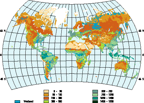
For present-day climate and soil data sets, NEM predicts an annual flux of 11.3 Tg-N (17.8 Tg N2O). This flux is at the high end of the IPCC (1994) estimate of the range for total N2O emissions from natural and cultivated soils of 5.1-15 Tg-N (8-23.6 Tg N2O). However, NEM may overestimate natural emissions because it uses a process model developed for managed ecosystems which may not be applicable to unmanaged ones. Figure 6 shows predicted present-day annual-average N2O emissions over the globe. Note that NEM predicts large emissions from tropical soils, which is qualitatively consistent with the observed latitudinal gradient for N2O (Prinn et al., 1990; Liu 1996), and in situ flux measurements (Keller and Matson, 1994).
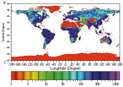
Figure 6 Predicted annual-average soil nitrous oxide emissions (gN/hectare/month) from Natural Emissions Model at 2.5 x 2.5o resolution.
As for TEM above, we have assessed the effect of driving NEM with the 2D-LO versus 3D climate models (Liu, 1996). We specifically use predicted climate and soil organic carbon from the three "doubled-CO2" climate model and TEM runs discussed earlier. Results are similar for global emissions driven by the three different climate models (2D-LO, GISS, GFDL), plus TEM scenarios. They indicate that equilibrium climate changes due to doubling CO2 would lead to a 32-40% increase in N2O emissions, even though soil organic carbon in TEM is reduced by 1.3% for these climate and CO2 changes. If correct, these results indicate a significant (positive) feedback between climate change and N2O emissions. For the "doubled CO2" experiment, the predicted temperature increases are the dominant contributor to increases in global N2O emissions.
The methane emission component in NEM is developed specifically for wetlands (Liu, 1996). For high latitude wetlands (i.e., northern bogs), NEM includes a hydrological model that solves a one-dimensional heat diffusion equation and water balance equation to predict bog soil temperature and moisture profiles, and water table position. An empirical formula, which uses the water table level and the bog soil temperature at this level, is then used to predict methane emissions. The hydrological model is driven by surface temperature and precipitation, which links methane emission with climate.
Data sets for the global distribution of wetlands and inundated areal fraction (Matthews and Fung, 1987) are used in the global emission model for methane. These data have 1o x 1o resolution. The above interactive emissions and climate model only applies to northern forested and nonforested bogs. NEM uses the averaged measured emission rates for tropical forested and nonforested swamps and alluvial formations, (Bartlett and Harriss, 1993), adjusted for temperatures differing from those during the measurements using the temperature dependence formula of Cao et al., (1995). This procedure leads to somewhat higher emissions than those computed using the rates from Fung et al. (1991).
Model predictions for present-day climate and wetland conditions are shown in Figure 7. The calculated global natural CH4 emission rate is 126.8 Tg CH4 per year, which is in the middle of the range of recent estimates for natural wetland emissions (Bartlett and Harriss, 1993; Reeburgh et al., 1993; IPCC, 1994). While tropical swamps and alluvial formations contribute 74.3 TgCH4/year, the northern bogs contribute 52.5 Tg/year. Driven by the above three "doubled- CO2" climates, CH4 emissions rise by 63% (2D-LO), 60% (GFDL), and 48% (GISS). This strong temperature dependence for CH4 emissions leads to a positive feedback similar to that for N2O.
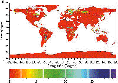
Figure 7. Predicted annual-average wetland CH4 emissions (109 g CH4/degree2/ month) from Natural Emissions Model at 1o x 1o resolution.
2.2.2 Oceanic fluxes
In order to model the oceanic sink of CO2, we adopt a dynamically simple and widely used scheme that incorporates a series of joined, interacting, carbon reservoirs (e.g., Oeschger et al., 1975; Bolin 1981; Ojima, 1992). Our so-called "Ocean Carbon Model" (OCM) is designed to be integrated interactively with the 2D-LO climate model and has several similarities to the models of Siegenthaler and Joos (1992), Stocker et al. (1994), Siegenthaler and Sarmiento (1993), Sarmiento et al. (1992), de Haan et al. (1994), and Matsuoka et al. (1995), except that the latter model predicts only global averages.
We assume that the air-sea flux of CO2 is proportional to the concentration gradient (which is dependent on solubility according to Henry's Law and hence temperature) multiplied by a piston velocity, which is itself a function of the surface wind speed (Liss and Merlivat, 1986; Tans et al., 1990). In the top layer of the ocean, additional dissolved CO2 is converted into bicarbonate (HCO3-) and carbonate (CO32-) ions to maintain a chemical equilibrium which is non-linearly dependent on mixed-layer temperature and alkalinity and atmospheric CO2 (see e.g., Peng et al., 1982; Goyet and Poisson, 1989). Changes in carbonate alkalinity allow equivalent acidity (or pH) to be explicitly predicted in the OCM, assuming current values of titration alkalinity and temperature dependent changes in the concentrations of boric, silicic, and phosphoric acids. This acid-base chemistry allows more CO2 to enter the mixed-layer than would be possible by solubility alone by delaying surface saturation with respect to CO2. Note that this approach automatically accounts for the significant sensitivity of the Revelle buffer factor to temperature, alkalinity, and CO2 concentrations (Takahashi, 1980).
Together, CO2, HCO3-, and CO32- (collectively called total dissolved inorganic carbon, DIC) are assumed to be transported away from the top layer and into the deep ocean as an inert tracer. Using the same reference values for these diffusion coefficients as used for computing perturbations to heat fluxes in the 2D-LO Climate Model (Section 2.4), the OCM achieves the same global CO2 uptake by the ocean as a 3D ocean GCM in an experiment with prescribed increases in atmospheric CO2 and no climatic feedbacks to circulation (Sarmiento and Quéré, 1996). For the purposes of this sensitivity study, we choose a magnitude for these diffusion coefficients which reproduces the oceanic CO2 uptake estimated by the IPCC (1994) for the 1980s of about 2 GtC/yr. This choice requires diffusion coefficients a factor 1.5 times larger for DIC than for heat fluxes. The factor of 1.5 produces a modest 15% increase in the global oceanic vertical CO2 flux. As a result of different controlling processes, the gradients and spatial scales for DIC and oceanic temperature perturbations are different. Hence we do not expect equality in DIC and heat diffusion coefficients. We caution that while biological effects are implicit in our chosen DIC diffusion coefficients, we do not explicitly include them. Sarmiento and Quéré (1996) showed that even a simple representation of biological processes leads to significant increases in the downward biogenic flux with time in a global warming simulation.
The OCM operates on the same horizontal grid scale as the 2D-LO Climate Model (Section 2.4), with 22 latitudinal oceanic zones from 90oN to 74oS. Vertically, for each latitude zone, the model has an atmospheric boundary layer (essentially the lowest atmospheric layer over the ocean in the 2D-LO model) and an oceanic mixed layer whose thickness is equal to the annual mean thickness of the mixed layer from the 2D-LO model, and which varies (increases) with latitude. Beneath the oceanic mixed layer, is a deep ocean diffusive layer running from the bottom of the mixed layer to a depth of 3000 meters. This diffusive layer is divided into 10 sub-layers (excluding the mixed layer) of increasing thickness for the purposes of numerical integration, which yields vertical profiles of DIC concentrations with depth. The vertical diffusion coefficients employed are constant with depth but variable with latitude, and are 1.5 times those used for heat transport in the 2D-LO model as noted above. Horizontal diffusion coefficients, which are a function of depth, but the same at all latitudes, are included to simulate horizontal CO2 transport by the thermohaline circulation and other processes. Values were chosen for these coefficients leading to pole-to-pole transport times of about 25 years in the upper ocean and 500 years in the lower ocean. Sensitivity studies show that the rate of CO2 uptake is insensitive to factor of 5 or less variations in these horizontal diffusion coefficients over the time-scales of the simulations.
The OCM is driven by inputs from the 2D-LO chemistry/climate model (described in Sections 2.3 and 2.4), namely the partial pressure of CO2 in the atmospheric boundary layer, ocean mixed layer temperature, and the magnitude of the horizontal surface wind velocity. The latter velocity is the same as that used for ocean-atmosphere heat exchange in the 2D-LO climate model, which is augmented from the velocity explicitly predicted to account for unresolved large-scale eddies. Values of the ocean-atmosphere exchanges and oceanic CO2 fluxes are computed on a daily basis as functions of latitude in the OCM. Exchange occurs in all areas free of sea ice as predicted in the 2D-LO model.
The (non-equilibrium) oceanic DIC distributions for the initial year (1977) for the runs shown here were obtained by running the OCM for 212 years from a calculated oceanic state in 1765 which was in equilibrium with preindustrial CO2 concentrations (278 ppm). This transient run was driven by observed or inferred (ice core) atmospheric CO2 levels for 1765-1977 and the 1765-1977 climate predicted by the 2D-LO model. Predicted present-day distributions of DIC in the deep ocean using the chosen DIC diffusion coefficients compare reasonably well with observations (Broecker and Peng, 1982; Brewer et al., 1986).
2.3 Atmospheric Chemistry | top of page |
For atmospheric composition predictions we use a coupled two-dimensional
atmospheric chemistry/climate model. This is a finite difference model on
latitude-pressure coordinates, and the continuity equations for trace
constituents are solved in mass conservative or flux form (Wang et al.,
1995, Wang, Prinn, and Sokolov, 1998). The local trace species tendency is thus
a function of convergence due to two-dimensional advection, parameterized
north-south eddy transport, and convective transports, and local true
production or loss due to surface emission or deposition and atmospheric
chemical reactions.
The atmospheric chemistry model includes 25 chemical species including
CO2, CH4, N2O, O3, CO,
H2O, NOx, HOx, SO2, sulfate aerosol
and chlorofluorocarbons. There are 41 gas-phase and 12 heterogeneous reactions
(Table II). The continuity equations for CFCl3,
CF2Cl2, N2O, O3, CO,
CO2, NO, NO2, N2O5,
HNO3, CH4, CH2O, SO2, and
H2SO4 include convergences due to transport whereas the
remaining very reactive atoms, free radicals, or molecules in Table II are
assumed to be unaffected by transport because of their very short lifetimes.
Water vapor and air (N2 and O2) mass densities are
computed using full continuity equations as a part of the climate model to
which the chemical model is coupled. The latter model also provides wind
speeds, temperature, solar radiation flux and precipitation which are used in
the chemistry formulation.
Table II. Gaseous and Aqueous Phase Chemical Reactions Included in the Model.
No. |
Reactions | References for Rate Constants |
| R1 | O3 + hv O(1D) + O2 | DeMore et al., (1994) |
| R2 | O(1D)+ H2O 2OH | DeMore et al., (1994) |
| R3 | O(1D) + N2 O + N2 | DeMore et al., (1994) |
| R4 | O(1D) + O2 O + O2 | DeMore et al., (1994) |
| R5 | CO + OH H + CO2 | Atkinson et al., (1992) |
| R6 | H + O2 + M HO2 + M | Atkinson et al., (1992) |
| R7 | HO2 + NO OH + NO2 | DeMore et al., (1994) |
| R8 | NO2 + hv NO + O | DeMore et al., (1994) |
| R9 | O + O2 + M O3 + M | Atkinson et al., (1992) |
| R10 | HO2 + O3 OH + 2O2 | Atkinson et al., (1992) |
| R11 | OH + O3 HO2 + O2 | Atkinson et al., (1992) |
| R12 | NO + O3 NO2 + O2 | Atkinson et al., (1992) |
| R13 | NO2 + OH + M HNO3 + M | Atkinson et al., (1992) |
| R14 | NO2 + O3 NO3 + O2 | DeMore et al., (1994) |
| R15 | NO3 + NO2 + M N2O5 + M | Atkinson et al., (1992) |
| R16 | HO2+ HO2 H2O2 + O2 | DeMore et al., (1994) |
| R17 | H2O2 + hv 2OH | DeMore et al., (1994) |
| R18 | H2O2+ OH HO2 + H2O | Atkinson et al., (1992) |
| R19 | HO + HO2 H2O + O2 | Atkinson et al., (1992) |
| R20 | HO + HO H2O + O | Atkinson et al., (1992) |
| R21 | HO + HO + M H2O2 + M | Atkinson et al., (1992) |
| R22 | CH4 + OH CH3 + H2O | Atkinson et al., (1992) |
| R23 | CH3 + O2 + M CH3O2 + M | Atkinson et al., (1992) |
| R24 | CH3O2 + NO CH3O + NO2 | DeMore et al., (1994) |
| R25 | CH3O + O2 CH2O + HO2 | Atkinson et al., (1992) |
| R26 | CH3O2 + HO2 CH3O2H + O2 | DeMore et al., (1994) |
| R27 | CH3O2H + hv CH3O + OH | DeMore et al., (1994) |
| R28 | CH3O2H + OH CH3O2 + H2O | DeMore et al., (1994) |
| R29 | CH2O + hv CHO + H | DeMore et al., (1994) |
| R30 | CH2O + OH CHO + H2O | Atkinson et al., (1992) |
| R31 | CHO + O2 CO + HO2 | Atkinson et al., (1992) |
| R32 | SO2 + OH + M HOSO2 + M | Atkinson et al., (1992) |
| R33 | HOSO2 + O2 HO2 + SO3 | DeMore et al., (1994) |
| R34 | SO3 + H2O H2SO4 | Atkinson et al., (1992) |
| R35 | CFCl3 + O(1D) products | DeMore et al., (1994) |
| R36 | CFCl3 + hv products | DeMore et al., (1994) |
| R37 | CF2Cl2 + O(1D) products | DeMore et al., (1994) |
| R38 | CF2Cl2 + hv products | DeMore et al., (1994) |
| R39 | N2O + hv N2 + O(1D) | DeMore et al., (1994) |
| R40 | N2O + O(1D) 2NO | DeMore et al., (1994) |
| R41 | N2O + O(1D) N2 + O2 | DeMore et al., (1994) |
| R42 | H2SO4(g) H2SO4(aq) | Pandis and Seinfeld (1989) |
| R43 | H2SO4(aq) HSO4- + H+ | Pandis and Seinfeld (1989) |
| R44 | HNO3(g) HNO3(aq) | Pandis and Seinfeld (1989) |
| R45 | HNO3(aq) NO3- + H+ | Pandis and Seinfeld (1989) |
| R46 | CH2O(g) CH2O(aq) | Pandis and Seinfeld (1989) |
| R47 | SO2(g) SO2(aq) | Pandis and Seinfeld (1989) |
| R48 | SO2(aq) HSO3- + H+ | Pandis and Seinfeld (1989) |
| R49 | HSO3- SO3= + H+ | Pandis and Seinfeld (1989) |
| R50 | H2O2(g) H2O2(aq) | Pandis and Seinfeld (1989) |
| R51 | HO(g) HO(aq) | Pandis and Seinfeld (1989) |
| R52 | HO2(g) HO2(aq) | Pandis and Seinfeld (1989) |
| R53 | HO2(aq) H+ + O2- | Pandis and Seinfeld (1989) |
In its present form the chemical model uses specified stratospheric photochemical destruction rates computed off-line in a global 3D stratospheric model (Golombek and Prinn, 1986; 1993). The model at present does not consider non-methane hydrocarbons but a simplified treatment of these is planned for future versions. The advection scheme is fourth-order positive-definite (Wang and Chang, 1993; Wang and Crutzen, 1995) and is used in a time-splitting procedure to calculate advection in each spatial dimension in order. Then a non-oscillatory scheme is used to limit numerical errors induced by possible spurious estimates of fluxes. Finally, a mass adjustment for correcting the error induced by time-splitting and possible non-convergence-free wind fields is used. The set of ordinary differential equations for the chemical reactions is stiff (see e.g., Brasseur and Madronich, 1992). To address this, a modified version of the LSODE code (Hindmarsh, 1983) is used.
The chemical model is run almost fully interactively with the 2D-LO climate model (Wang et al., 1995; Wang, Prinn, and Sokolov, 1998). The model computes the zonal-means of predicted species concentrations over land and ocean (or both) on the 24 latitudinal by nine vertical layers (seven tropospheric and two stratospheric) grid of the 2D-LO model. The time stepping for the chemistry is 20 minutes for advection, one hour for physics (other than radiation), and three hours for photochemistry. The chemistry and climate dynamics are fully interactive: every five hours the calculated radiative forcing is updated by the predicted concentrations of CO2, CH4, N2O, chlorofluorocarbons, and sulfate aerosol. Aerosols can also affect radiative forcing indirectly through increasing the reflectivity of water clouds. This indirect aerosol effect is poorly understood and highly uncertain (IPCC, 1996a; Hansen et al., 1997). Following IPCC (1996a) we assume somewhat arbitrarily that indirect aerosol radiative forcing is twice the calculated direct radiative forcing. We examine sensitivity of results to aerosol radiative forcing assumptions later. North-south transport in the coupled model, which is based on predicted winds and a parameterized eddy transport scheme, was tested using the chlorofluorocarbon CFCl3. Industrial CFCl3 emissions were input at the surface, and predictions compared very well with ALE/GAGE observations (Cunnold et al., 1994) including the north-south intrahemispheric and interhemispheric gradients (Figure 8) thus providing confidence in the model transport schemes. Sample outputs from this model for O3 (a greenhouse gas), and SO2 (the precursor for sulfate aerosols) are shown in Figure 9. While further improvements are planned, the current version provides a reasonably good simulation of observed distributions of CH4, CO, and O3 (Wang, Prinn, and Sokolov, 1998), and predicts OH concentrations and distributions in reasonable agreement with those derived from CH3CCl3 (Prinn et al., 1995). OH is the major species removing CH4, CO, SO2, and NOx from the atmosphere.
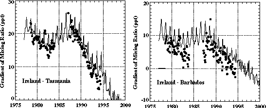
Figure 8. Time evolution of the lat-itudinal gradient of surface
CFCl3 mixing ratio, defined as the differences between mixing ratios
at Ireland (52oN) and Tasmania (40oS) [upper graph], and
between mixing ratios at Ireland and Barbados (13oN) [lower graph], for
the model (solid lines) and observations (dots).
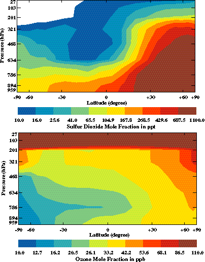
Figure 9. Predicted monthly-mean distributions of the SO2 mixing
ratio (ppt) and O3 mixing ratio (ppb) in December 1995 from
chemistry model as a function of latitude (degrees, positive for North and
negative for South), and pressure (hPa = millibar).
2.4 Climate Dynamics | top of page |
As noted earlier, climate dynamics is addressed using a two-dimensional (2D) land-ocean-resolving (LO) statistical-dynamical model (Sokolov and Stone, 1995, 1997a, b). It is a modified version of a model developed at the Goddard Institute for Space Studies (GISS) (Yao and Stone, 1987; Stone and Yao, 1987 and 1990). Unlike energy balance models usually used in sensitivity studies and in many integrated assessment models (IPCC 1990, 1992 and 1996a; Murphy, 1995; Matsuoka et al., 1995; Wigley and Raper, 1993; Jonas et al., 1996), the 2D-LO model explicitly solves the primitive equations for zonal mean flow and includes parameterization of heat, moisture, and momentum transports by large scale eddies based on baroclinic instability theory. It also includes parameterizations of all the main physical processes such as radiation, convection, and cloud formation. As a result, it is capable of reproducing many of the nonlinear interactions taking place in GCMs.
Since the original version of the 2D model was developed from the 3D GISS GCM (Hansen et al., 1983), the model's numerics and parameterizations of physical processes are closely parallel to those of this GCM. The grid used in the model consists of 24 points in latitude (corresponding to a resolution of 7.826 degrees) and, in the standard version, nine divisions in the vertical (two in the planetary boundary layer, five in the troposphere, and two in the stratosphere). The number of vertical divisions can be varied. The important feature of the model, from the point of view of coupling chemistry and climate dynamics, is that it incorporates the radiation code of the GISS GCM. This code includes all significant greenhouse gases, such as H2O, CO2, CH4, N2O, chlorofluorocarbons, and ozone, and 11 types of aerosols.
The land-ocean resolving 2D-LO model, like the 3D GISS GCM, allows up to four different kinds of surface in the same grid cell; namely, open ocean, ocean-ice, land, and land-ice. The surface characteristics (e.g., temperature, soil moisture) as well as surface turbulent fluxes are calculated separately for each kind of surface while the atmosphere is assumed to be well mixed horizontally in each grid cell. The weighted averages of fluxes from different kinds of surfaces are used to calculate changes of temperature, humidity, and wind speed in the model's first layer due to air-surface interaction.
Two fundamentally different types of clouds are taken into account in the model: convective clouds, associated with moist convection; and large-scale or supersaturated clouds, formed due to large-scale condensation. Since anthropogenic sulfate aerosols are mainly concentrated over land, the radiative fluxes are calculated separately over land, ocean, and sea-ice.
The 2D-LO model includes a mixed-layer ocean model. In order to simulate the current climate, the equation for the mixed-layer temperature includes a term representing the effect of horizontal heat transport in the ocean and heat exchange between the mixed layer and deep ocean. This model is somewhat simpler than that of de Hann et al. (1994) which resolves the Atlantic and Pacific oceans. The 2D-LO ocean horizontal heat flux would equal the observed ocean heat transport if the model were perfect (i.e., if no "flux adjustment" common in coupled ocean-atmosphere GCMs were needed). In fact, the 2D-LO model simulates quite well the observed ocean heat transport in the Southern Hemisphere (in contrast to some GCMs, see Gleckler et al., 1995), but overestimates somewhat the heat transport in the Northern Hemisphere.
In simulations of transient climate change the heat uptake by the deep ocean has been parameterized by diffusive mixing driven by perturbations of the temperature of the mixed layer, into deeper layers (Hansen et al., 1988). The zonally averaged values of diffusion coefficients calculated from measurements of tritium (Table III) are referred to as "standard" ones hereafter. The global average value of the vertical diffusion coefficients (Kv) is 2.5 cm2/s for these standard values. However, Hansen et al. (1984, 1997) found that an equivalent value of Kv that gives similar results when used in a 1D model is only 1 cm2/s. As will be shown below, a doubling of the standard diffusion coefficients is required to match the behavior of the "upwelling diffusion-energy balance" (UD-EB) model used in IPCC (1996a). The UD-EB model uses a diffusion coefficient equal to 1 cm2/s, but also takes into account upwelling with a hypothesized decrease in the upwelling rate due to slow-down of the thermohaline circulation induced by a global warming.
Table III. Coefficients of heat diffusion into the deep ocean (cm2/s).
| Northern hemisphere | |||||||||||
| 90oN |
82oN |
74oN |
66oN |
59oN |
51oN |
43oN |
35oN |
27oN |
20oN |
12oN |
4oN |
| 0.76 |
1.44 |
3.31 |
4.63 |
5.14 |
3.57 |
2.57 |
1.62 |
1.34 |
0.54 |
0.22 |
0.23 |
| Southern Hemisphere | |||||||||||
| 4oS |
12oS |
20oS |
27oS |
35oS |
43oS |
51oS |
59oS |
66oS |
74oS |
82oS |
90oS |
| 0.32 |
0.43 |
1.24 |
1.53 |
2.61 |
4.67 |
6.97 |
7.60 |
8.11 |
9.73 |
0.00 |
0.00 |
Using the predicted rates of increase in oceanic temperatures and the equation of state of seawater, we also calculate the rate of change of global average sea level due to thermal expansion of the ocean following the method described by Gregory (1993). For this purpose, observed data (Levitus, 1982) are used for the "unperturbed" state of the deep ocean. Note that the greater the rate of heat transport into the ocean, the slower the rate of surface temperature rise, but the greater the rate of oceanic thermal expansion.
A significant number of simulations of present climate have been performed with the 2D-LO model (Sokolov and Stone, 1995, 1997a). Zonal wind and specific humidity (winter and summer) for the 2D-LO model are both in reasonable agreement with observations (Peixoto and Oort, 1992). Accurate prediction of specific humidity is important for both radiation (H2O is a greenhouse gas) and chemistry (H2O is a source of OH). Both the 2D-LO and GISS models in general have difficulty matching the observed precipitation, but the 2D-LO model performs reasonably well in the tropics. In any case, there are significant disagreements among observational data sets for precipitation. The pattern of evaporation is also reasonably well reproduced by the 2D-LO model. The 2D-LO model does not reproduce well the seasonal cloud change in the tropics associated with the shift of the Intertropical Convergence Zone because of its low latitudinal resolution. Otherwise, the overall pattern of seasonal cloud changes simulated by the 2D-LO model is quite similar to the observed one (Schiffer and Rossow, 1985; Hahn et al., 1988). The same is true for the seasonal change in cloud radiative forcing (Ramanathan et al., 1989). Finally, the treatment of horizontal oceanic heat transport in the GISS GCM and 2D-LO models (see above) ensures good simulations of observed global sea surface temperatures (Oort, 1983). Both models also provide good simulations of observed global tropospheric temperatures.
In summary, a comparison of the model's results with the observational data shows that it reproduces reasonably well the major features of the present climate state. Of course, there are important longitudinally varying phenomena that cannot be simulated by a 2D model. However, the depiction of the zonally averaged circulation by the 2D-LO model is not very different from that by 3D GCMs. Since the model is to be used for climate change prediction, it is noteworthy that the seasonal climate variation is also reproduced quite well.
When using a 2D model to study uncertainty in climate change, it is desirable to have a model capable not only of simulating the present climate but also of reproducing the climate change pattern obtained in simulations with different coupled ocean-atmosphere GCMs. Versions of the model with different sensitivities were formulated by inserting an additional cloud feedback, in the way proposed by Hansen et al. (1993). Specifically, the calculated cloud amount is multiplied by the factor (1+k d Ts), where d Ts is an increase of the global averaged surface air temperature with respect to its value in the present climate simulation. The predicted increase in equilibrium surface air temperature due to a doubling of the CO2 concentration by current GCMs ranges from 1.9 to 5.4oC. A significant reason for this wide range is related to differences in cloud feedbacks produced by different GCMs (Cess et al., 1990; Senior and Mitchell, 1993; Wetherald and Manabe, 1988; Washington and Meehl, 1989, 1993). That, in turn, is caused mainly by different treatments of cloud optical properties. The feedback associated with changes in the optical properties of clouds is, of course, different from that associated with the changes in cloud amount used in our simulations. However, different versions of the 2D-LO model reproduce well the results from various GCM runs for the relationships between surface warming and increase in precipitation (Figure 10), and between surface warming and changes in components of the surface heat balance (Sokolov and Stone, 1997a).
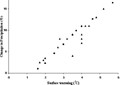
Figure 10. Percentage change in globally and annually averaged pre-cipitation as a function of equilibrium global mean sur-face warming caused by a doubling of CO2 as predicted by different GCMs (triangles; from IPCC, 1990) and different versions of the 2D-LO model (circles).
In general, responses of different versions of the 2D-LO model to the doubling of CO2, in terms of both global average and zonal mean temperatures, are similar to those obtained in simulations with different GCMs (Sokolov and Stone, 1997a). Since the climate model outputs are used in the simulations with the TEM, it is important to note that insertion of the additional cloud feedback described above, while allowing us to change model sensitivity, does not lead to any physically unrealistic changes in climate. On the contrary, changes in other climate variables, such as precipitation, and evaporation are also consistent with the results produced by different GCMs (Sokolov and Stone, 1997a).
The transient behavior of different GCMs can be matched by choosing appropriate values for the model's sensitivity and the rate of heat diffusion into the deep ocean (Sokolov and Stone, 1997a, b). The change in the latter was obtained by multiplying the standard diffusion coefficients (Table III) by the same factor at all latitudes, thereby preserving the latitudinal structure of heat uptake by the deep ocean. The time-dependent global averaged surface warming produced by different versions of the 2D-LO model are compared with the results of the simulations with the GFDL, Max-Planck Institute (MPI), and National Center for Atmospheric Research (NCAR) GCMs in Figures 11 and 12. The transient response of the 2D-LO model with doubled standard ocean heat uptake is similar to those obtained in the simulations with the GFDL GCM with different rates of CO2 increase (Figure 11; IPCC, 1996a). Ten times standard values of the diffusion coefficients are required to match the delay in warming produced by the MPI GCM (Figure 12; Cubasch et al., 1992). Data for the MPI model have been modified to take into account effects in that model of its "cold start" (Hasselman et al., 1993). At the same time, essentially no heat diffusion into the deep ocean in the 2D-LO model is required to reproduce the fast warming produced by the NCAR GCM (IPCC, 1996a). Since the UD-EB model used in IPCC (1996a) was tuned to reproduce the global averaged results of the GFDL GCM, it has a rate of heat uptake close to that for the 2D-LO model with doubled diffusion coefficients.
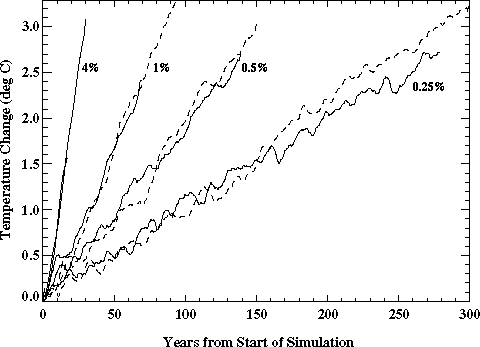
Figure 11. Global mean surface air temperature change caused by a 4%, 1%, 0.5%,
and 0.25% per year increase in CO2 in the simulations with the 2D-LO
model with a sensitivity of 3.7oC and Kv=5.0 cm2/s
(solid curves) and the GFDL GCM (dashed curves, R. Stouffer, private
communication, 1996).
Figure 12. Global mean surface air temperature change caused by prescribed
increases in CO2 in the simulations with the MPI and NCAR GCMs
(dashed curves) and in the matching versions of the 2D-LO model (solid curves).
Prescribed increases are 1% per year for the NCAR model and IPCC IS92(A) and
(D) for the MPI model. 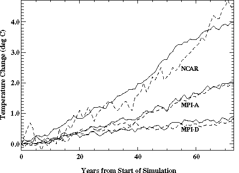
The only significant difference between results of the 2D-LO model and the GFDL GCM occurs in the simulation with 0.25% per year increase in CO2. The difference is significant only after some 120-150 years of integration. Aside from that, the various versions of the 2D-LO climate model reproduce quite well the globally averaged surface warming predicted by different GCMs (GFDL; GISS; NCAR; MPI; Murphy and Mitchell, 1995) for a variety of forcing scenarios. At the same time, there is no strong interhemispheric asymmetry in the transient warming simulated by the 2D model, in contrast with the results produced by most of the GCMs cited here. However, some recent studies show that current ocean models may produce excessive vertical mixing in high latitudes of the Southern Hemisphere and that, as a result, the corresponding retardation of warming predicted by GCMs in the Southern Hemisphere may be exaggerated (IPCC, 1996a).
Another characteristic describing changes in the deep ocean temperature is sea level rise due to thermal expansion. In spite of our model's simplified representation of the deep ocean, it reproduces very well the thermal expansion of the deep ocean as simulated by the GFDL GCM (Figure 13), except again for the simulation with 0.25% per year increase in CO2.
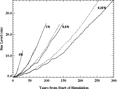
Figure 13. Global mean sea level rise due to thermal expansion caused by a 4%, 1%, 0.5%, and 0.25% per year increase in CO2 in the simulations with the 2D-LO model with a sensitivity of 3.7oC and Kv=5.0 cm2/s (solid curves) and the GFDL GCM (dashed curves, R. Stouffer, private communication, 1996).
2.5 Terrestrial Ecosystems| top of page |
As noted earlier, we predict global ecosystem states using TEM (Raich et
al., 1991; McGuire et al., 1992; 1993; 1995; Melillo, 1994; Melillo
et al., 1993; 1995; Xiao et al., 1997). The TEM is a
process-based ecosystem model that simulates important carbon and nitrogen
fluxes and pools for 18 terrestrial ecosystems. It runs at a monthly time step.
Driving variables include monthly average climate (precipitation, mean
temperature and mean cloudiness), soil texture (sand, clay and silt
proportion), elevation, vegetation and water availability. The water balance
model of Vorosmarty et al. (1989) is used to generate hydrological input
(e.g., potential evapotranspiration, soil moisture) for TEM. For global
extrapolation, TEM uses spatially-explicit data sets at a resolution of
0.5o latitude by 0.5o longitude (about 55 km x 55 km at the equator).
The global data sets include long-term average climate (updated version of
Leemans and Cramer, 1991 and Cramer and Leemans, 1993; W. Cramer, personal
communication), potential natural vegetation (Melillo et al., 1993),
soil texture (FAO/CSRC/MBL, 1974) and elevation (NCAR/Navy, 1984). These data
sets contain 62,483 land grid cells, including 3,059 ice grid cells and 1,525
wetland grid cells. Geographically, the global data sets cover land areas
between 56oS and 83oN.
Net primary production (NPP) is an important variable in climate change impact
assessment. In TEM, NPP is calculated as the difference between gross primary
production (GPP) and plant (autotrophic) respiration (RA). The GPP
monthly flux is calculated as a function of the maximum rate of C assimilation,
photosynthetically active radiation, leaf area relative to maximum annual leaf
area, temperature, atmospheric CO2 concentration, water
availability, and nitrogen availability (Raich et al., 1991). The
monthly flux RA, which includes both maintenance respiration and
construction respiration of higher plants, is calculated as a function of
temperature and vegetation carbon.
Using TEM Version 4.0 (McGuire et al., 1995, 1997; Pan et al.,
1996; Xiao et al., 1995, 1996a, b, 1997), which has a number of advances
over earlier versions, we previously estimated global annual NPP to be 47.9
PgC/yr when ecosystems are in equilibrium under "contemporary" climate with 315
ppmv CO2 (Xiao et al., 1995, 1996a, b, 1997). This was in the
middle of the range of 13 other estimates (Melillo, 1994; Potter et al.,
1993; Whitaker and Likens, 1973). NPP in tropical regions was estimated to be
as much as two times higher than NPP in temperate regions (Figure 14) in this
equilibrium state. Tropical evergreen forests accounted for 34% of
global NPP, although their area is only about 14% of the global land area used
in the simulations. Tropical ecosystems (tropical evergreen forest, tropical
deciduous forest, xeromorphic forest and tropical savanna) accounted for 57% of
global NPP. NPP was low in high-latitude ecosystems in the northern hemisphere,
where NPP was primarily limited by low temperature and nitrogen availability.
Polar desert/alpine tundra and moist tundra ecosystems occur over 8% of the
global land area but accounted for only 2% (0.9 PgC/yr) of global NPP.
Together, boreal forests and boreal woodlands accounted for 14.5% of the global
land area and their annual NPP was about 8% (3.9 PgC/yr) of global NPP. NPP in
arid regions accounted for 4% of global NPP, although the area of arid regions
is about 20% of the global land area.
Figure 14. Estimates of Net Primary Production (NPP) (gC/m2/yr) for
CO2 levels of 315 ppm and contemporary climate defined by long-term
mean climate data (Cramer and Leemans, 1993; W. Cramer, private communication).
These previous TEM runs indicated that global NPP (and total carbon storage
discussed earlier in Section 2.2.1) increases substantially for the change from
the above equilibrium with contemporary climate (with 315 ppmv CO2)
to an equilibrium with a perturbed climate (with 522 ppmv CO2).
However, the predicted NPP increase varies little among equilibrium climate
change predictions from the three climate models: +17.8% for the 2D-LO model
climate change, +18.5% for the GFDL GCM climate change, and +20.6% for the GISS
GCM climate change. Generally, the latitudinal distribution of NPP change under
the 2D-LO model climate change is similar to those under the GISS and GFDL GCM
climate changes, except for relatively large differences within the 50.5oN
to 58.5oN and 66.5oN to 74oN bands associated with differences
in cloudiness and temperature within these two bands in the three climate
predictions (Xiao et al., 1996a, b, 1997). Note that NPP at these
latitudes is only a fraction of the global total, so differences here do not
yield significant global differences.
For climate change impact assessment, spatial aggregations of changes of NPP
for potential vegetation for the 12 economic regions in EPPA provide a
potential linkage between the projection of anthropogenic emissions, their
impacts on terrestrial ecosystems, and the subsequent feedback on potential
agricultural performance. For each of the 12 EPPA economic regions, TEM
estimates of annual NPP for equilibrium conditions increase substantially and
about equally for the above three equilibrium climate change predictions (Table
IV). India, the Dynamic Asian Economies (DAE) and energy exporting developing
countries (EEX) have relatively smaller responses of annual NPP. Note that for
the geographically disconnected EPPA regions (OOE, EEX, ROW), this aggregation
may mask important effects in individual countries. For most economic regions,
the predicted increases of annual NPP are slightly smaller under the 2D-LO
model climate change than under the GISS and GFDL GCM climate changes.
Table IV. Changes from "today's" values of equilibrium annual NPP and
total carbon storage due to changes in equilibrium climate and indicated
atmospheric CO2 concentrations for the 12 economic regions in EPPA
(Xiao et al., 1996b). See Table 1 for definitions of regions.
| Annual Net Primary Production |
Total Carbon Storage | ||||||||
| CO2 level: |
315 ppmv |
522 ppmv |
315 ppmv |
522 ppmv | |||||
| Climate scenarios: |
Contemp. |
MIT L-O |
GISS |
GFDL-q |
Contemp. |
MIT L-O |
GISS |
GFDL-q | |
| Economic Regions |
area (106 km2) |
(PgC/yr) |
(%) |
(%) |
(%) |
(PgC/yr) |
(%) |
(%) |
(%) |
| USA |
9.1 |
3.2 |
22.6 |
23.3 |
20.0 |
118 |
9.1 |
9.2 |
5.6 |
| Japan |
0.4 |
0.3 |
21.7 |
20.4 |
28.6 |
9 |
12.5 |
12.2 |
17.4 |
| India |
3.1 |
1.2 |
11.6 |
15.3 |
17.6 |
35 |
6.0 |
8.0 |
10.4 |
| China |
9.4 |
3.6 |
17.9 |
18.6 |
23.1 |
131 |
8.8 |
7.7 |
11.6 |
| Brazil |
8.2 |
6.3 |
15.9 |
16.9 |
14.8 |
6 |
15.9 |
16.9 |
14.8 |
| EEC |
2.4 |
1.3 |
23.6 |
23.5 |
22.6 |
45 |
13.5 |
13.2 |
11.2 |
| EET |
1.1 |
0.6 |
24.6 |
24.4 |
20.8 |
22 |
13.8 |
13.1 |
9.7 |
| DAE |
1.0 |
0.8 |
11.2 |
11.4 |
12.5 |
22 |
6.7 |
5.9 |
8.1 |
| OOE |
20.0 |
4.7 |
23.2 |
25.1 |
22.7 |
231 |
7.1 |
8.6 |
8.0 |
| FSU |
21.1 |
4.2 |
20.8 |
28.0 |
28.1 |
296 |
-0.6 |
9.0 |
8.0 |
| EEX |
22.5 |
9.4 |
15.9 |
19.2 |
15.7 |
255 |
9.1 |
9.4 |
8.7 |
| ROW |
32.1 |
12.4 |
16.0 |
19.8 |
15.7 |
330 |
7.6 |
7.9 |
6.6 |
Similarly, the responses of total carbon storage are close to each other among the three climate change predictions for most economic regions. An exception is the former Soviet Union (FSU) region, where total carbon storage decreases slightly (-0.6%) under the 2D-LO model climate change, but increases 8.0% under the GFDL GCM climate change and 9.0% under the GISS climate (Table IV). As noted above, this difference is caused in large part by the higher temperature and cloudiness changes in the high latitudes in the predicted 2D-LO model climate change. These comparisons indicate that the 2D-LO climate model yields, for the most part, similar results to 3D models for impact assessment based on NPP at the scale of the EPPA economic regions. Of course, this similarity by itself is by no means a reason for confidence in either the 2D or 3D models.
In the initial versions of TEM, including Version 4.0 used by Xiao et al. (1995, 1996b) in the studies with the 2D-LO and other climate models, both input and output variables are assumed to represent equilibrium conditions. In equilibrium, the annual fluxes of carbon, nitrogen, and water into the terrestrial ecosystem equal annual fluxes of these compounds out of the ecosystem (e.g., annual NPP = annual heterotrophic respiration (RH) so that annual NEP = 0.0). Thus, seasonal carbon, nitrogen, and water dynamics within a year can be examined, but transient interannual dynamics of carbon, nitrogen, and water cannot be simulated. For applications such as inclusion in the IGSM, a new version of TEM (Version 4.1) has been developed that can determine transient estimates of important carbon and nitrogen fluxes of terrestrial ecosystems based on transient CO2 concentrations and transient climate variables. The equilibrium assumption allowed variables such as photosynthetically active radiation, soil moisture, and relative leaf area to be estimated by intermediate models before initiating a TEM run (Pan et al., 1996). To develop TEM Version 4.1, the algorithms of these intermediate models have been incorporated into TEM so that all seasonal variables except air temperature, precipitation, and cloudiness are calculated concurrently each month. This new version of TEM can be used in either transient mode or equilibrium mode.
When Version 4.1 is run in transient mode, there is no requirement that annual fluxes of carbon, nitrogen, and water into the terrestrial ecosystem equal annual output fluxes. Hence a non-zero NEP estimate is possible and NEP (i.e., net carbon exchange between atmosphere and land biosphere) can increase or decrease in response to transient climate change. For global extrapolation of a transient simulation, Version 4.1 uses the same global data sets of potential vegetation, soil texture, and elevation described earlier, and the transient carbon dioxide, surface temperature, precipitation, and cloudiness estimates derived from the coupled chemistry/climate model (Section 2.4) model to simulate interannual dynamics of carbon, nitrogen, and water. This latest version, run in transient mode, is used in all the runs described in the following sections. To initialize these runs, TEM Version 4.1 was run from assumed equilibrium conditions in 1765 to a non-equilibrium condition in 1976 driven by the 1765 -1976 climate calculated using the 2D-LO model, with both TEM and the 2D-LO model being driven by the same observed CO2 history as used for the OCM initialization.
2.6 Coupled Model Interfaces | top of page |
The component models in the IGSM are formulated with different spatial
resolutions and integrating time steps and so they must be harmonized at the
component model interfaces. First, the predicted emissions from the 12 economic
regions of the EPPA model are converted into emissions at the 24 latitude grid
points (7.826o resolution) of the chemistry/climate model. This is done
using a mapping procedure which takes into account the number of latitude grid
points spanned by each economic region and allocates the emissions in each
region by the fraction of its population contained in each latitude band (Liu,
1994). EPPA is solved in five-year time steps, and emissions into the chemistry
model (which is run on 20-, 60-, and 180-minute time steps) are interpolated
values which are updated every year. Future versions of EPPA will include
treatments of seasonal variations in emissions, which are substantial for some
gases.
Since the atmospheric chemistry and climate models are run interactively and
simultaneously, they are already fully harmonized in space and time. The
climate model (which is integrated in 20-minute time steps) supplies monthly
average climate variables to TEM. These monthly averages are zonal values over
land at 7.826o latitudinal resolution; they are used to adjust the
corresponding variable of the contemporary (observed) climate used in TEM, thus
producing "perturbed" climates at the needed 0.5o latitude by 0.5o
longitude resolution. A similar mapping procedure produces monthly-average
climate variables for input into the natural N2O and CH4
emission (NEM) models (which have 2.5o x 2.5o and 1o x 1o
horizontal resolutions, respectively). Finally, TEM variables required in the
NEM N2O model are aggregated to the appropriate resolution and input
as monthly averages. These mapping procedures, using longitudinal model
averages and observed climate patterns, bear some similarity to that used by
Jonas et al. (1996) which involves global mean model values and
predicted climate patterns in a general circulation model. As demonstrated by
Jonas et al. (1996), such procedures are useful but give different
results for different GCMs.
For the reference run discussed here, and the sensitivity runs discussed
below, the TEM model was not yet capable of being coupled interactively with
the chemistry/climate model. Hence it was run non-interactively after the
chemistry/climate model integrations. In order to include CO2 uptake
by terrestrial ecosystems in the chemistry/climate model we therefore used a
very simple parameterization in which this rate of uptake (B) is constant.
Values for B are determined from values predicted for current oceanic
CO2 uptake in the OCM and current CO2 emissions from EPPA
using the constraint that the model simulate currently observed CO2
trends. Similarly, we assumed that the natural emissions of CH4 and
N2O were constant at values necessary to simulate current trends of
these two gases given the EPPA estimates of anthropogenic emissions and
chemistry model estimates of loss rates. We assume a constant natural
production of SO2 (mainly from oxidation of dimethyl sulfide of
oceanic origin) of 12.8 TgS/yr. For technical reasons, we also assumed constant
ozone levels in the radiation calculations in the 2D-LO model rather than those
predicted in the chemistry model itself (future versions will use the predicted
ozone concentrations). Once the TEM runs were complete, we then were able to
test the validity of these simple assumptions and to assess the importance of
including TEM and ozone interactively in order to address feedbacks. The NEM
model was run both non-interactively after the chemistry/climate and TEM model
runs and also interactively with the chemistry/climate model.
3. RESULTS FROM A REFERENCE RUN | top of page |
A sample integration, referred to as a "reference" run, of the IGSM is used to
illustrate the nature of the interactions among component sub-models. The
"reference" run consists of a sequential integration of EPPA (Section 2.1), the
coupled 2D-LO chemistry/climate/ocean carbon model (Sections 2.2.2, 2.3, 2.4),
TEM (Section 2.5), and NEM (Section 2.2.1). This reference run is not intended
to be a "best estimate" prediction, although it is also not intended to be an
"extreme" prediction. This run incorporates a run of EPPA which
produces CO2 emissions similar to those assumed in the IPCC IS92a
scenario (IPCC, 1992) and lying in the mid-range of estimates from integrated
assessments (Edmonds, Wise, and Barns, 1995). It also uses a version of the
2D-LO climate model which has a sensitivity to doubled CO2 that is
near the center of the range of models reviewed in IPCC (1996a) and a rate of
heat uptake by the ocean similar to that of the UD-EB model of the IPCC
(1996a). Finally, this run includes a treatment of sulfate aerosols produced
from anthropogenic SO2 emissions. Thus this reference run, while not
a "best estimate", is a convenient case for comparison with model results of
other researchers and is a suitable baseline for the sensitivity analysis
described in Section 4.
3.1 Model Results | top of page |
In the EPPA model reference run, the processes that lead to changes in
emissions can be summarized in terms of the growth in economic activity and
(using CO2 as an example) the carbon intensity of that activity, as
illustrated earlier in Figure 3. The main cause of the overall increase in
global CO2 emissions in the reference case is growth in regional
gross domestic product (GDP), as shown in Table V. As indicated in the last
column of the Table, regional differences in predicted GDP growth are large.
The differences reflect assumptions regarding population growth and increases
in labor productivity, as well as differences in capital formation. The
resulting predicted global emissions for CO2 and other gases are
shown by the solid lines in Figure 15. These emissions are added to estimates
of natural emissions (dotted lines in Figure 15) which, as already noted, are
assumed to remain constant in the reference run.
Figure 15. Annual EPPA (solid lines) and natural (dotted lines)
emissions for the Reference Run.
Table 5. Changes in Regional DGP, Reference Case
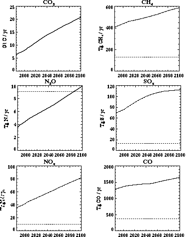
1985 GDP |
Growth Rates of Regional GDP |
GDP in 2100 | |||||
| Region |
(billion 1985 US$) |
1985-2000 |
2000-2025 |
2025-2050 |
2050-2075 |
2075-2100 |
as a multiple of 1985 |
| USA |
3,692.54 |
2.70% |
1.86% |
1.43% |
1.24% |
0.99% |
5.9 |
| JPN |
1,265.99 |
3.48% |
2.81% |
1.62% |
1.24% |
0.99% |
8.7 |
| EEC |
2,227.56 |
2.85% |
1.99% |
1.25% |
0.78% |
0.58% |
4.8 |
| OOE |
787.41 |
3.25
% |
1.92% |
1.39% |
1.14% |
0.90% |
6.1 |
| EEX |
1,047.61 |
6.62% |
3.32% |
1.79% |
1.08% |
0.84% |
14.9 |
| CHN |
440.90 |
9.19% |
3.87% |
2.70% |
1.76% |
1.11% |
38.3 |
| FSU |
637.74 |
3.95% |
3.20% |
1.97% |
1.67% |
1.43% |
13.8 |
| IND |
181.79 |
8.78% |
4.74% |
2.96% |
1.98% |
1.43% |
54.3 |
| EET |
237.15 |
1.81% |
3.51% |
1.89% |
1.61% |
1.30% |
10.2 |
| DAE |
261.78 |
6.94% |
4.89% |
2.78% |
1.48% |
0.86% |
32.0 |
| BRA |
186.31 |
1.59% |
3.25% |
1.76% |
0.80% |
0.41% |
5.9 |
| ROW |
614.24 |
3.16% |
2.62% |
1.76% |
1.14% |
0.86% |
7.7 |
The coupled 2D atmospheric chemistry and 2D-LO climate model, initialized with 1977 composition observations, was then run for the 1977-2100 year time period. The climate model has time-invariant "background" aerosols as defined in the parent NASA/GISS 3D model (Hansen et al., 1983, 1984). The reference run includes anthropogenic sulfate aerosols (which are added to the background) produced by the predicted anthropogenic SO2 emissions. The output as a function of latitude and time for temperature, precipitation, cloudiness, and CO2 from the coupled 2D chemistry/climate model, are then used to drive the transient version of TEM. Finally, the predictions of total soil carbon from the transient TEM are combined with the climate model predictions of temperature and precipitation to drive NEM.
The results from the reference run for globally averaged CO2, temperature change, precipitation change, cloudiness change, sea level change, total NPP change, total NEP, and natural emissions are shown in Figure 16. We express changes with respect to a 1990 because FCCC discussions usually reference emission reductions to this particular year. The predicted increases in precipitation (both globally and in the Northern Hemisphere in particular) serve to increase the rate of removal of sulfate aerosol in the coupled model; this is a feedback not included in uncoupled models. Also, note that the 2D-LO climate model shows interannual variations of about 0.06oC, 3.5 mm/yr, and 0.28% in globally averaged temperature, precipitation, and cloudiness, respectively (Figure 16) and these variations are reflected in variations in NPP and NEP. Between 1990 and 2100 both net primary production (NPP) and heterotrophic respiration (RH) rise significantly. The difference (NEP or net CO2 exchange) increases from 0.81 (1990) to 2.6 (2100) PgC/yr (GtC/yr). Hence our assumption of a constant B=2.1 GtC/yr was inconsistent with the trend but not with the average of predicted NEP. As noted in Section 2.5, these runs of the transient TEM are initiated using non-equilibrium conditions in 1976. While these are preliminary calculations, and need further careful analysis, uptake of CO2 by land ecosystems is predicted to be very significant. Also, the fertilization effect of rising CO2 and predicted increases in precipitation and decreases in cloudiness over land are sufficient, apparently, to offset ecosystem stresses induced by rising temperatures, at least in a global aggregate.
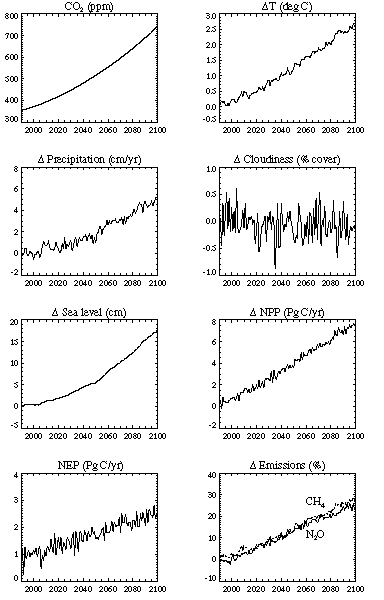
Figure 16. Predictions from the global system model for either the global-total or global-average values, or the changes in these values from their 1990 levels, are given for CO2 concentrations, surface air temperature, precipitation, cloudiness, sea level, net primary production, net ecosystem production, and natural N2O and CH4 emissions as a function of time for the reference run.
Natural soil emissions of N2O rose about 25% between 1990 and 2100, and wetland CH4 emissions rise by 28%. These increases result from the sensitivity of wetland CH4 emissions to the predicted large high-latitude temperature increases (and modest precipitation increases), and the sensitivity of the global soil N2O emissions to temperature and rainfall increases and to changes in labile soil carbon. Our results for N2O are qualitatively similar to those of Alcamo et al. (1996). These effects need to be further examined and validated. Nevertheless, it appears that these positive feedbacks should be considered in coupled models. In particular, given these results, it appears that our assumption in the reference run that natural CH4 and N2O emissions are constant is not valid. Using a version of the IGSM in which NEM is run interactively with the chemistry and climate models, the N2O and CH4 concentrations were both 6% higher in 2100 relative to the reference.
For the purposes of this experiment, the OCM was first run from "pre-industrial times" (assumed to be 1765) in which the oceanic mixed layer and the deep ocean are considered to have been in equilibrium with the atmosphere at a constant CO2 mixing ratio of 278 ppmv. The net carbon flux between atmosphere and ocean is therefore zero in 1765, and all oceanic concentrations are in equilibrium with pre-industrial ocean temperature and alkalinity profiles. The OCM was driven by historical CO2 concentrations as estimated from Greenland ice core data for 1765-1957, and Mauna Loa, Hawaii measurements between 1958 and 1977. Climate variables for 1765-1977, such as temperature and surface wind speeds, were from a run of the 2D-LO model driven by the same historical CO2 concentrations. Then, from 1977 onward, the OCM was run fully interactively with the 2D-LO climate/chemistry model. The results, which are discussed in more detail in Section 4, indicate that rising CO2 concentrations in the atmosphere drive a flux of carbon into the ocean that grows from about 2.5 GtC/year in 1990 to 8.8 GtC/year in 2100.
The scientific usefulness of the simplified 2D-LO chemistry/climate model is evident from this reference run. It allows quantification of several important feedbacks between climate, chemistry (e.g., aerosol removal), ecosystems (e.g., CO2 uptake), and natural emissions (e.g., of N2O and CH4). We can in the future test the robustness of these conclusions by performing many more runs of this computationally efficient model, with different assumptions in the sub-model components for comparison with observations. Such extensive testing would not be practical with a global system model incorporating a 3D chemistry/climate model. We emphasize again that this run should not be regarded as a "best estimate". It is simply a "reference" case dependent on assumptions made in the EPPA, natural emissions, atmospheric chemistry, climate, and terrestrial ecosystem models.
3.2 Latitudinal Variations | top of page |
As noted earlier, the capability of the MIT model to resolve processes by
latitude is important both for scientific and policy purposes. The predicted
latitudinal variations are driven by the dependence on latitude of both
anthropogenic emissions (from EPPA) and natural climate, chemistry, and
ecosystem processes (in the chemistry/climate model, OCM, TEM, and NEM). The
evolution in the reference run of the surface concentrations of CO (an air
pollutant), O3 (a greenhouse gas and air pollutant) and OH (an
indicator of the intensity of the atmospheric oxidizing rate) are shown as
functions of latitude and time in Figure 17. Significantly, the global average
OH concentration fell by about 20% between 2000 and 2100 thus increasing the
lifetime of CH4 by the same percentage. This lowering of OH is
associated with the growth in CH4 and to a lesser extent CO, both of
which consume OH. Figure 18 illustrates the latitudinal evolution of the
concentration of NOx (a pollutant and, after conversion to nitrate,
a potential ecosystem nutrient), the concentration of anthropogenic
SO2 (a pollutant), and the vertical optical depth of
H2SO4 aerosol (a measure of aerosol cooling by sunlight
reflection, and also a pollutant and potential ecosystem nutrient).
Figure 17. Temporal evolution of the annual-mean surface air con-centrations of
CO (upper panel, in ppb), O3 (middle panel, in ppb), and OH (lower
panel, 10-3 ppt) as functions of lat-itude (in degrees, denoted as
positive in Northern Hemi-sphere, negative in Southern Hemisphere) in the
reference run.
Figure 18. As in Figure 17, but for NOX (upper panel, in ppt),
anthropogenic SO2 (middle panel, in ppb), and
H2SO4 vertical optical depth (lower panel, actual
dimensionless values are multiplied by 100 for display here).
Notable from Figures 17 and 18 for all atmospheric species except OH are the
increases with time at each latitude and the extension of the regions of high
pollutant levels from the northern hemisphere mid-latitudes into the northern
hemisphere sub-tropics (and to a lesser extent into the southern hemisphere).
This behavior is expected because of the predicted increasing global emissions
(Figure 15) and the geographic shifts of these emissions (see Section 2.1) in
the EPPA model. However, ozone concentrations (Figure 17) show only modest
(roughly 10%) increases over this time period. Recall that we assume constant
(current day) tropospheric ozone levels to compute radiative forcing in the
reference run so this assumption is evidently not an important source of error.
Ozone levels are a complex function of the NOx, CO, CH4,
and HOx levels, and further discussion of these results is provided
elsewhere (Wang et al., 1997). Note however that because these predicted
concentrations are averaged over longitude, actual concentrations in industrial
regions of the short-lived species depicted in Figures 17 and 18 will be
significantly higher than indicated. We are currently developing algorithms
using EPPA, population data, and a simplified mesoscale air pollution model
(Calbo et al., 1998) to incorporate a better treatment of regional air
pollution in the IGSM.
It is important to consider spatial variations in radiative forcing (Hansen
et al., 1997). The time evolution of the changes in latitudinal
distributions of radiative forcing relative to 1990, both
longitudinally-averaged over ocean and land and longitudinally-averaged over
land only, are shown in Figure 19. Clearly evident is the steady increase in
radiative forcing with time due to the rising CO2, CH4,
and N2O concentrations. Another prominent feature is the influence
of the negative radiative forcing due to the direct and indirect effects of
rising aerosol levels, particularly over land in the northern hemisphere
(15oN-50oN). Specifically, in the 2050-2100 period there is about a
20-year lag between changes in radiative forcings over land and ocean at
30oN and the corresponding forcing northward of 60oN and southward of the equator. For the forcing over land only, the lag is 40 years.
Figure 19. Changes in longitudinally-averaged radiative forcing
(watt/m2) from 1990 levels for land and ocean (upper panel), and
land only (lower panel), are given as functions of latitude (in degrees, with
positive values in Northern Hemisphere and negative values in Southern
Hemisphere) and time (in years).
These predicted patterns of radiative forcing manifest themselves in a complex
way as changes in surface temperature as a function of latitude and time over
land and ocean (see Figure 20). The 2D-LO climate model predicts much more
rapid rises in temperature in polar than in tropical regions, and over land
compared to ocean, in general agreement with 3D climate models. The regional
effects of the negative forcing by aerosols are more subtle, apparently causing
a delay in warming in the northern extratropics compared to the southern
extratropics of only about a decade. Evidently, the greater delay in warming
caused by the greater ocean area in the southern hemisphere offsets somewhat
the greater cooling caused by the much higher anthropogenic aerosol levels in
the northern hemisphere. In addition, the aerosols significantly reduce the
rate of increase of the global-average temperature as discussed in the
sensitivity runs in the following section. These results are qualitatively
similar to those obtained in recent transient general circulation model runs
incorporating both greenhouse gas and direct and indirect aerosol effects
(Meehl et al., 1996). Note however that our 2D-LO model cannot simulate
potential regional changes attributed to the aerosols, such as the weakening of
the South Asian Monsoon evident in the Meehl et al. (1996) results.
Figure 20. As in Figure 19 but for surface temperature change (oC) over land and ocean (upper panel) and over land only (lower panel).
When used to drive TEM, the predicted climate and CO2 changes
produce complicated time variations of net primary production and net ecosystem
production. Various runs of TEM have been carried out to determine sensitivity
to the predicted changes in CO2, temperature, precipitation, and
cloudiness, each considered separately. Neglecting nonlinear interactions,
these runs indicate that global NPP changes are driven primarily by the rising
CO2 levels and secondarily by the temperature increases. Predicted
reductions in cloudiness (and to a lesser extent temperature increases) appear
to lower NPP, while rising precipitation increases it. Global NEP behavior is
dominated by a competition between rising CO2 (which raises NPP and
yields a positive NEP) and rising temperature (which raises RH and
yields a rapidly varying negative NEP). Precipitation and cloudiness changes
produce rapid interannual NEP variations, but little long-term effects.
The latitudinal variations in NPP and NEP, shown in Figure 21 show different
responses by tropical and mid-latitude ecosystems to the imposed climate and
CO2 changes. Both NPP and NEP rise steadily in mid-latitude
ecosystems, while tropical ecosystems initially have rapidly rising positive
NEP, and later declining NEP. These differences have implications for the
differential distribution of impacts among countries. For policy purposes, NPP
variations in the 12 EPPA regions provide a useful qualitative measure of
changes in natural ecosystem state and potential agricultural production
resulting from climate change (Figure 22). Note that NPP is predicted to
increase in all EPPA regions.
Figure 21. Longitudinally-cumulative terrestrial NEP (upper panel) and NPP
(lower panel) predicted as a function of latitude (in degrees with positive
denoting North and negative denoting South) and time (in years) in the
transient TEM reference run. Units are TgC/yr (MtC/yr) for each 0.5 degree
latitude band.
Figure 22. Predicted changes in NPP from their 1990 levels in the 12 EPPA
economic regions as a function of time (in years) in the transient TEM
reference run. Units are PgC/yr (GtC/yr).
Changes with time in latitudinal patterns of natural emissions of
N2O and CH4 predicted in NEM are small, consisting simply
of an expansion of the range of latitudes for strong tropical and boreal
CH4 emissions and boreal N2O emissions. Runs of NEM
driven by climate change alone, and by climate plus total soil carbon changes
(the latter from TEM), show that climate changes (rising temperatures and
rainfall) and soil carbon increases (about 9% between 1990 and 2100) contribute
about equally to the predicted 28% rise in N2O emissions (Figure 16).
4. SENSITIVITY ANALYSIS| top of page |
Sensitivity analyses help identify those specific components of models which
most affect the important model outputs. For this purpose, we have carried out
a series of runs of the MIT model in which key parameters or assumptions in the
component sub-models are varied by finite amounts from their values in the
reference run discussed in the previous section. Finite changes are employed
because we have no a priori expectation that the coupled model response to
these changes is linear and, at the same time, computational constraints limit
exploration of the degree of non-linearity involved. The "brute-force"
(non-local) sensitivity so-defined is a function potentially of the magnitude
of the assumed changes and is time dependent because of the lags between
forcing and response in the IGSM.
In these tests we focus on sensitivity to variation within the EPPA and
coupled 2D-LO chemistry/climate models, and the design of the experiment is
shown in Figure 23. For the EPPA model and each of the two key components of
the 2D-LO climate/chemistry model (chemistry and climate dynamics) a
three-point range of assumptions is chosen. In each case one of these runs is
the "reference" discussed above, and it is denoted "R" in the figure and in the
discussion to follow. The two other cases are designed to yield results which
are "higher" (denoted H) and "lower" (denoted L) than the reference for some
key model output. For the EPPA model, the key output is total CO2
emissions over the analysis period; for the other two components the key output
is the global mean temperature in 2100.
Figure 23. Schematic illustrating the runs performed for the sensitivity
analysis of the IGSM. Open circles denote points in sequence where output is
available, with the letters in the circle denoting the identifying symbol for the output.
Definition of the H and L cases involves a priori identification of one
or two of the most important assumptions that are uncertain in the particular
sub-model, based on the judgment of the experts in charge of it. The variables
and the values chosen are presented in Table VI. For EPPA emissions, the
critical assumptions involve the treatment of labor productivity growth (which
drives overall economic growth, and is treated as a surrogate for the joint
effect of population and productivity change), non-price-induced changes in
energy efficiency (the AEEI), and backstop technology costs. For atmospheric
composition, assumptions selected as especially significant include the rates
of terrestrial and oceanic uptake of CO2 and the influence of
anthropogenic sulfate aerosols. As summarized in Table VI, the rate of
terrestrial CO2 uptake is imposed as a constant rate B in each run
and oceanic uptake is a function of the assumed vertical diffusion
coefficients. The uncertainty in the influence of aerosols is addressed by an
adjustment to the calculated aerosol optical depths. Critical assumptions for
climate dynamics involve the treatments of convection and clouds (which effect
the model sensitivity to doubled CO2) and the rates of oceanic heat
uptake (determined like CO2 by the vertical diffusion coefficients).
The sensitivity analysis is facilitated by the capability for altering the
cloud feedback and ocean mixing rates specially built into the 2D-LO model
(Section 2.4).
Table VI. Summary of assumed values for uncertain parameters in the EPPA
and coupled chemistry/climate models in the sensitivity analysis.
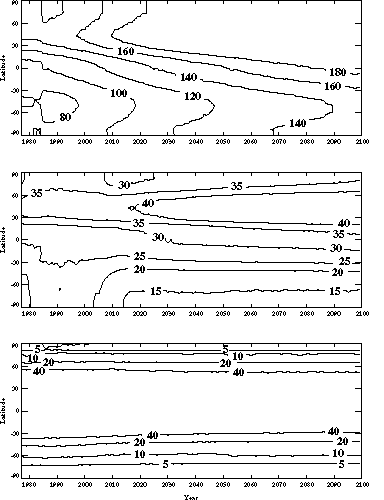
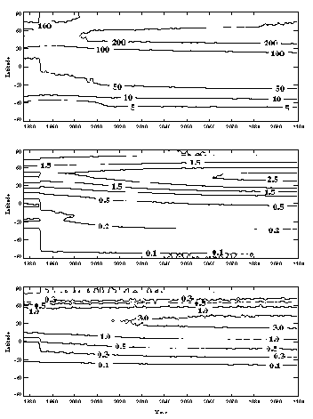
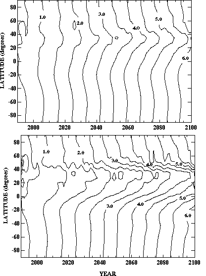
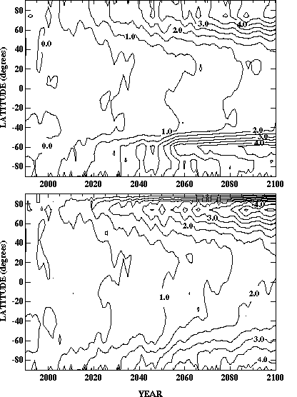
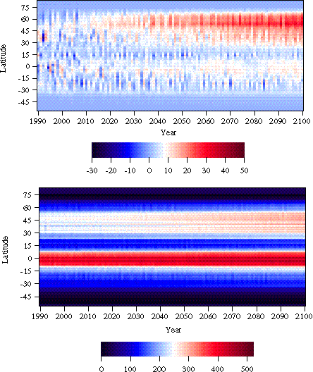
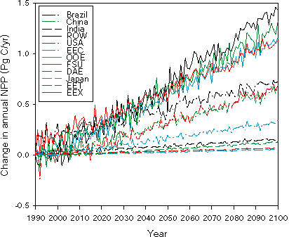
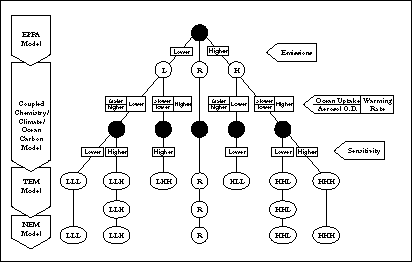
Output Variable |
Effect on Output Variable | |||
| EPPA |
Lower |
Ref |
Higher | |
| Labor Prod. (%/yr)1 |
Emissions (2100) |
0.8, 1.6 |
1,2 |
1.25, 2.50 |
| AEEI (%/yr) |
1.4 |
0.75 |
0.25 | |
| Non-C backstop (cents/Kwh) |
10 |
15 |
22.5 | |
| Chemistry/Climate |
Lower |
Ref |
Higher | |
| Land C Uptake2 B (GtC/yr) |
Temp. (2100) |
1.1 |
2.1 |
3.1 |
| Ocean Diff. Coef.3 (multiplier) |
10 |
2 |
0.4 | |
| Aerosol Opt. Dep.4 (multiplier) |
2 |
1 |
0.5 | |
| Sensitivity5 (oC) |
2.0 |
2.5 |
3.5 | |
|
1 End point (2100) labor productivity rates are shown, with rate for
OECD and EEX given first and other regions given second. 2 Carbon uptake by the terrestrial biosphere and oceanic diffusion coefficients are not independent choices. Faster oceanic CO2 uptake caused by larger diffusion coefficients must be accompanied by lower terrestrial CO2 uptake to fit current CO2 observations. 3 Standard oceanic vertical diffusion coefficients (Table III) are multiplied by the given factor for heat and 1.5 times the given factor for carbon in each case. Fast oceanic heat and CO2 uptake which result from higher diffusion coefficients combine to lower rate of warming and vice-versa. 4 Calculated optical depths (direct plus indirect) are multiplied by the given factor to account for uncertainty in predicted aerosol concentrations, optical properties, and cloud nucleation effects. Aerosol optical depth significantly affects temperature and sea level when this factor exceeds unity but not when this factor is less than unity. 5 Defined as difference in global average surface temperature between equilibrium climates for current and doubled CO2 levels and strongly dependent on model cloud treatment. | ||||
Several considerations influenced the choice of the assumed parameter values in Table VI. In this construction the rate of terrestrial biospheric carbon uptake (B) is not independent of the oceanic diffusion coefficients which effect oceanic uptake. Values chosen for B and the diffusion coefficients must lead to agreement with current CO2 observations, so that the setting of one determines the level of the other. This condition holds despite the fact that the two phenomena are not obviously linked in a physical or biological sense. Also, although no formal uncertainty analysis is attempted here, an effort is made to seek a rough comparability of the uncertainties attributed to each of the three stages in the sensitivity analysis (emissions, aerosol forcing combined with ocean diffusion, and climate sensitivity, as shown in Figure 23). For each stage, parameter values for the "higher" and "lower" cases were chosen such that, in the subjective judgments of the modelers, for given inputs there is roughly only one chance in three of the output from that particular stage lying outside the H-L range. The procedure is approximate, but it helps insure plausible choices for the input parameters.
This test of the three component models, with three choices each, leads to a total of 27 possible combinations. To limit the number of runs, a sub-set of seven sensitivity cases is chosen. Each is identified by a three-letter name indicating the emissions, aerosol/ocean, and cloud feedback parameter choices, in that order. The logic of the construction is the following. In addition to the reference case (RRR), two cases were selected (HHH and LLL) which define the overall range in terms of temperature change for the full 27 combinations. Next, two runs were selected to explore the range of response of NPP within the TEM model. It was expected that high NPP changes would result from a high level of CO2 and moderate temperature changes (HHL), and that low NPP changes would be found with low levels of CO2 and again moderate temperature changes (LLH). Finally, two cases are included, HLL and LHH, which assist in sorting out the relative influence of emissions, atmospheric chemistry, and climate dynamics. Thus the relative influences of CO2 uptake rates and anthropogenic emissions can be studied with a comparison of the differences between HHL and HLL (only the uptake varies) and between HHH and LHH (only the emissions vary). Similarly, the relative roles of anthropogenic emissions and chemistry/climate processes can be seen by a comparison of the differences between HLL and HHH (same emissions, different chemistry/climate) and those between HHH and LHH (same chemistry/climate, different emissions).
The combinations of assumptions concerning labor productivity, AEEI, and cost of non-carbon backstops in EPPA lead to changes in the evolution of economic structure over the century. Economic growth rates, which are influenced by all these assumptions as well as by the response of capital investment, differ among the cases. In the H case the GDP in China and India grows by 2100 to levels roughly 14% higher than under the reference (R) conditions shown in Table IV, and to levels 13% lower under the L assumptions. GDP in the OECD regions ranges up to 10% above and below the reference level in the H and L cases respectively. Also, the carbon intensity of economic activity changes. In the reference case, shown in Figure 3, the global energy intensity of economic activity drops from 460 MtC per US$ in 1985 to around 180 MtC in 2100. Under case L, it falls to 145 Mt per US$, but under the assumptions for the H case it falls only to 212 GtC in 2100.
The resulting emissions of climatically important gases are shown in Figures 24 and 25. Also shown is the IPCC (1992) IS92a scenario. Compared to IS92a, the range of EPPA predictions is lower for SO2 because, as noted earlier, control commitments by several countries are taken into account. The results are higher for CH4 and CO, and similar for N2O and NOx. Emissions predictions for most gases are sensitive to the economic assumptions applied in this analysis. The predicted lower (L) and higher (H) CO2, SOx, NOx, CH4, and N2O emissions in particular differ by 5 to 25% from the reference (R) run. In the current EPPA formulation, CO predictions vary only slightly in response to the three parameters chosen for testing. Note that the CO2 emissions in Figure 24 are augmented by deforestation emissions (Section 2.1.1), while the SO2, N2O and CH4 emissions in Figures 24 and 25 are augmented by constant natural fluxes of 12.8 TgS/yr, 9.1 TgN/yr, and 130 Tg CH4/yr, respectively.
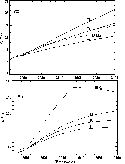
Figure 24. Higher (H), lower (L), and reference (R) CO2 emissions
(PgC/yr, GtC/yr) (upper graph) and SO2 emissions (TgS/yr) (lower
graph) from EPPA runs and IS92a IPCC (1992) emission scenarios. See Figure 23
for run nomenclature.
Figure 25. As for Figure 24 but for emissions of CH4 (Tg
CH4/yr), N2O (TgN/yr), CO (TgCO/yr), and Nox
(TgN/yr). See Figure 23 for run nomenclature.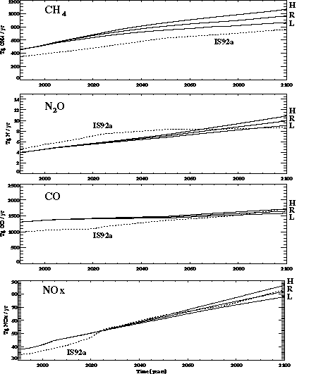
Mixing ratios of selected greenhouse gases from the seven runs of the coupled chemistry/climate model are shown in Figure 26. Note that CO2 mixing ratios are about equally sensitive to assumptions concerning oceanic (and the linked land biospheric) CO2 uptake rates (see e.g., differences between HHL and HLL runs or LHH and LLH runs) and assumptions concerning anthropogenic emissions (see e.g., differences between HHH and LHH runs or HLL and LLL runs). In contrast, CH4 mixing ratios are less sensitive to assumptions concerning climate which affects its chemical removal (see e.g., difference between HLL and HHH runs or LLL and LHH runs) than to assumptions about anthropogenic emissions (measured by HHH-LHH and HLL-LLL differences). Chemical removal of N2O is unaffected by climate in our current model so mixing ratios are sensitive only to anthropogenic emissions. However these conclusions concerning CH4 neglect the significant uncertainty in predicting OH (which destroys CH4). Also, for both CH4 and N2O, they neglect the effect of climate change on natural emissions (which as already noted were predicted to increase about 28% and 25%, respectively, in the reference run).
Figure 26. Predicted CO2 (ppm), N2O (ppb), CH4 (ppm); and CCl3F (ppt) mixing ratios for the seven sensitivity runs of the coupled chemistry/climate model. Emissions and hence mixing ratios of the chlorofluorocarbon CCl3F are the same in all seven runs. See Figure 23 for run nomenclature.
Sensitivity of the post-1990 changes of radiative forcing from 1990 values to the various model assumptions is shown in Figures 27 and 28. The change in total forcing from 1990 values is about equally sensitive to EPPA assumptions and aerosol/oceanic/biospheric uptake assumptions (i.e., HHL-HLL is similar to HHH-LHH, and LHH-LLH is similar to HLL-LLL). In the reference year (1990), the gas radiative forcing is essentially the same in all runs, but the aerosol radiative forcing for the HHH, HHL, and LHH runs is about 0.3 W/m2 less negative than in RRR while for the HLL, LLH, and LLL runs it is about 0.5 W/m2 more negative. These 1990 aerosol forcings (and to a lesser extent the post-1990 changes in Figure 27) are much more sensitive to assumptions about direct and indirect aerosol radiative effects than to EPPA assumptions influencing sulfur emissions (i.e., LHH-HHH is much less than HHL-HLL and LLL-HLL is much less than LHH-LLH). Changes in total radiative forcing between 1990 and 2100 plotted as functions of latitude (Figure 28) clearly show the cooling role of aerosols with the effects being most dramatic over land as expected. Note that the latitudinal pattern in aerosol forcing in the reference year of 1990 (not shown) maximizes around 40oN, while the changes after 1990 (shown in Figure 28) maximize around 30oN due to the southward spread of SO2 emissions with time.
Figure 27. Predicted changes in radiative forcing (exclusive of H2O)
from 1990 levels (W/m2) in the seven sensitivity runs. The upper
panel refers to all gases and aerosols and the lower panel to aerosols alone. See Figure 23 for run nomenclature.
Figure 28. Predicted changes (between 1990 and the average for 2090-2100) in
total radiative forcing (solid lines) and forcing due to gases only (dashed
lines) for the seven sensitivity runs. Upper panel refers to longitudinal
averages over land plus ocean and lower panel over land alone. Units are W/m2.
The responses of global average temperature and sea level to the changes in radiative forcing and to assumptions about climate model sensitivity are shown in Figure 29.Temperature change is about twice as sensitive to the chemistry/climate model assumptions (quantified by the difference between HHH and HLL or LHH and LLL) than to EPPA model assumptions (quantified by the difference between HHH and LHH or HLL and LLL). Assumptions about ocean uptake and aerosols (quantified by LHH-LLH) contribute about equally to assumptions about climate sensitivity (quantified by HHH-HHL) in the chemistry/climate model. The importance of the deep ocean circulation identified here is one impetus for our planned incorporation into the climate model of an improved (3D) ocean model with a more realistic treatment of ocean basins and the thermohaline circulation. Changes in the thermohaline circulation over time, which are not simulated here, can also have significant effects on climate (see e.g., Maier-Reimer et al., 1993; Marotzke and Stone, 1995; Manabe et al., 1991).
Figure 29. Changes in global-average surface air temperatures (upper panel, oC) and sea-level (lower panel, cm of rise due to ocean thermal expansion only) from 1990 values in the seven sensitivity runs.
Sea level rise (Figure 29) from oceanic thermal expansion depends on both surface temperature and the rate of oceanic diffusion. Specifically, the HHL run, which is warmer than the HLL run, shows about the same sea-level rise as HLL because of its slower oceanic diffusion. Note that the necessarily coherent changes in the rate of carbon and heat uptake by the ocean have opposite effects on sea level change. Larger heat uptake leads to greater sea level rise, but increased oceanic carbon uptake leads to lower radiative forcing and lower sea level rise. The net effect in the model is to decrease the sensitivity of sea level rise to oceanic vertical mixing (Sokolov et al., 1997c).
Latitudinal variations of surface air temperature change over land and land-plus-ocean show greatest sensitivity to model assumptions at high latitudes (Figure 30). The cooling effect of aerosols, most evident in the HLL, LLH, and LLL runs, leads to lower temperature changes in the Northern than in the Southern Hemisphere in these runs, despite the fact that they have faster oceanic heat uptake.

Figure 30. Changes (between 1990 and the average for 2090-2100) of longitudinally averaged surface air temperature (oC) over land plus ocean (upper panel) and land only (lower panel) for the seven sensitivity runs. Latitude in degrees, with positive values denoting Northern Hemisphere.
Longitudinally-averaged precipitation changes (Figure 31) in the tropics and mid-latitudes are much more sensitive to model assumptions than are changes in the sub-tropics and polar regions. The warmer model runs generally produce greater precipitation changes. Latitudinal patterns of cloudiness change (Figure 31) are sensitive to model assumptions in all regions, with the warmer model runs (HHH, LHH) showing very significant decreases in cloud cover. Note that these changes in cloud cover are influenced by the cloud feedback factor used to change the model sensitivity (Section 2.4).
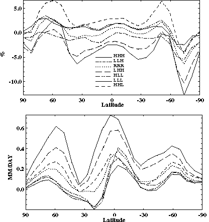
Figure 31. Changes (between 1990 and the average for 2090-2100) of longitudinally-averaged cloud cover (upper panel, % cover) and precipitation (lower panel, mm/day) over land for the seven sensitivity runs. Latitude in degrees, with positive values denoting Northern Hemisphere.
As noted earlier, three of the seven sensitivity runs (HHL, RRR, LLH) were chosen to drive the transient TEM. The results for global NPP, NEP, and reactive soil organic carbon are shown in Figure 32. Higher CO2 and slightly higher temperature changes (HHL) lead to higher increases in NPP, and lower CO2 and slightly lower temperature changes (LLH) lead to lower NPP increases. The NPP prediction, as already noted, is particularly sensitive to CO2 levels. Hence the differences between the three runs are explained in part by the differences in the CO2 levels in the HHL, RRR, and LLH cases which are similar before 2010 but diverge rapidly after that (Figure 26). The trends in NEP (Figure 32) also diverge for the three runs after 2010 (recall that NEP = NPP-RH, so this is not unexpected). Because NPP generally increases with CO2 concentrations and RH with temperature, the difference (which is carbon uptake by land ecosystems or NEP) ends up being larger for HHL than LLH. Therefore, the effect of the slightly higher temperatures on RH in HHL is more than offset by the effects of higher CO2 levels on NPP in the same run.
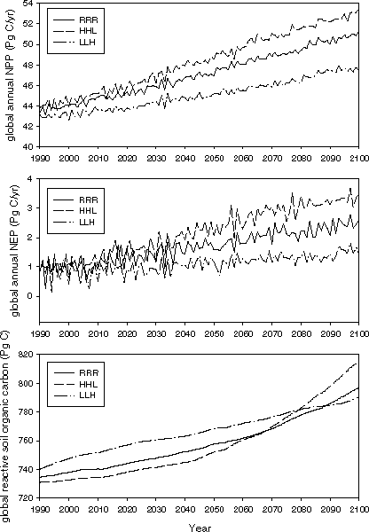
Figure 32. Global NPP (upper panel), NEP (middle panel), and reactive soil organic carbon (lower panel) predicted in transient TEM driven by the CO2 and climate variables from the reference and two selected sensitivity runs.
Reactive soil organic carbon (CR) is a function of litterfall production (and hence NPP) and heterotrophic respiration (and hence temperature), and is an important energy source for microorganisms involved in soil nitrogen cycling, including production of N2O. Up to about 2080, TEM estimates higher CR values (Figure 32) in the lower NPP/cooler climate (LLH) than in the higher NPP/warmer climate (HHL). The order then reverses after 2080. Changes in CR result from an imbalance of litterfall production (and hence NPP) and heterotrophic respiration (i.e., decomposition). As noted earlier, NPP is particularly sensitive to CO2 levels whereas heterotrophic respiration (RH) is sensitive to temperature variations. The transient responses of reactive soil organic matter to the three CO2 and climate time series indicates that CR is, as expected, sensitive to changes in both temperature and CO2 levels. With warmer temperatures, increased decomposition rates cause CR to decrease so that the cooler climate (LLH) has more CR than the warmer climate (HHL) in the early part of the transient when CO2 levels are more similar. However, the increases in CO2 concentration associated with the LLH climate begin to level off in the last 20 years of the run. This allows the resulting increases in RH to keep pace with the corresponding increases in NPP so that the amount of CR also begins to level off. In contrast, the more exponential increases in CO2 concentration associated with the HHL climate causes the increases in RH to lag the corresponding increases in NPP. The lag in response between RH and NPP then causes CR to increase. By the year 2080, the effect of enhanced CO2 on increased litterfall inputs has more than compensated for the effect of enhanced temperatures on decomposition.
Predicted emissions of N2O from runs of the NEM (Figure 33) indicate significant sensitivity to outputs from the climate (temperature, precipitation) and TEM (total soil carbon, CT) models. Two NEM reference runs driven by climate outputs only (denoted RRR) and reference climate plus TEM outputs (denoted RRR+CT) indicate that climate and soil carbon changes contribute about equally to the predicted very significant increase in N2O emissions (Figure 33). Methane emissions increase significantly and predictably with increasing temperature (c.f. Figure 29). Since soil carbon and temperature are predicted to change in all seven sensitivity runs, the importance of including the feedbacks to climate forcing involving changing natural emissions of N2O and CH4 is evident.
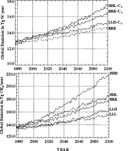
Figure 33. Predicted annual natural emissions of N2O (upper panel, TgN/year) and CH4 (lower panel, TgCH4/year) in NEM runs driven by the indicated climate model runs and (for N2O) also by the indicated climate plus TEM model runs (the latter denoted by the addition of CT to the run designation).
Finally, the OCM, which was run interactively with the chemistry/climate model, computed the net uptake of carbon by the ocean which increased in all runs (Figure 34). The OCM in the HLL, LLH, and LLL runs uses factor-of-five higher ocean diffusion coefficients than the reference, and predicts a larger oceanic sink in these three runs than the reference (RRR) run. Evidently, the effects of the lower CO2 emissions in the LLH and LLL runs relative to the reference are overwhelmed by the effects of the larger oceanic diffusion coefficients in these runs. Conversely, despite the higher CO2 levels in the HHL and HHH runs, the factor of five smaller diffusion coefficients lead to a smaller oceanic sink. The downward transport of carbon from the mixed layer (which saturates relatively quickly) is thus the limiting factor. The factor of five range in ocean diffusion coefficients was chosen because it is the range needed to simulate heat uptake by various GCMs (Section 2.4). Also, the predicted range in oceanic carbon uptake at the beginning (1977) of the seven OCM runs of 0.9 to 2.9 GtC/yr is in good agreement with the IPCC (1992) range. This provides further evidence of the plausibility of our chosen range for the diffusion coefficients. Finally, we tested the sensitivity of the OCM to the diffusion coefficients alone by changing them by factors of five or one-fifth, while holding the input CO2 predictions at their reference run values. Higher diffusion coefficients resulted in an increase in the OCM oceanic sink of about 34% in 2100 compared to the reference coefficients, while lower diffusion coefficients decreased the oceanic sink by about 47%.
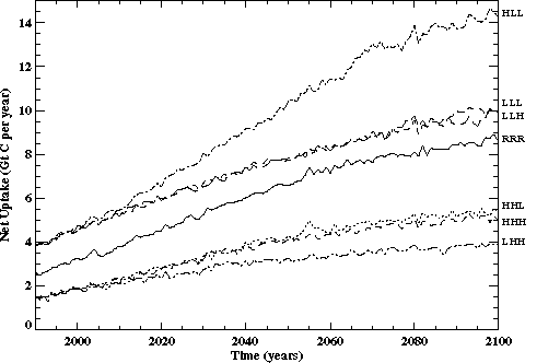
Figure 34. Predicted annual uptake rate of carbon (GtC/year) by the ocean predicted in the indicated OCM runs.
These results show that while the trend in the atmospheric concentration of CO2 determines the trend in uptake, the rates of diffusion in the deep ocean dominate in determining the magnitude of the flux of CO2 into the ocean. This sensitivity is also evident from the work of Sarmiento and Quéré (1996), who show that a weakening or collapse of the oceanic thermohaline circulation (equivalent to decreasing ocean diffusion coefficients with time in our model) leads to substantial reduction in oceanic CO2 uptake. This sensitivity of uptake to uncertain ocean mixing rates has considerable implications for estimating the anthropogenic emissions necessary to reach particular target CO2 concentrations in the atmosphere.
5. SUMMARY AND CONCLUSIONS| top of page |
We have developed a comprehensive Integrated Global System Model for climate
science and policy analysis. It consists of coupled sub-models of economic
growth and associated anthropogenic emissions (EPPA), natural N2O
and CH4 fluxes (NEM), interactive atmospheric chemistry and climate
(2D-LO model), and natural terrestrial ecosystems (TEM). It addresses many of
the major anthropogenic and natural processes involved in climate change and is
also computationally efficient. As such, it can be used to study parametric and
structural uncertainty and to analyze costs and impacts of multiple policy
proposals. From a selected set of runs of this global system model we have
obtained the following results:
(1) We have identified and quantified a number of potentially important
feedbacks between the sub-models. Between chemistry and climate, these
feedbacks include changes in precipitation affecting aerosol removal rates, and
changes in water vapor and temperature affecting atmospheric oxidation rates.
Between land ecosystems, the carbon cycle, and climate, the feedbacks include
changes in climate and CO2 influencing net ecosystem production
(NEP) and thus CO2 uptake rates by these ecosystems. Specifically,
the NEP changes which occur in response to CO2 changes may provide a
negative feedback in the carbon cycle similar to that provided by the ocean.
Yet to be included and quantified is the feedback of net primary production
(NPP) onto agriculture and thus economic development. Finally, natural
emissions of CH4 and N2O are predicted to increase
substantially with increasing temperature and precipitation, providing a
positive feedback between climate and the CH4 and N2O
cycles.
(2) We have demonstrated a potential for significant future changes in the
magnitudes and geographical distribution of anthropogenic emissions,
concentrations of greenhouse gases, aerosols and pollutants, radiative forcing,
temperature (and other climate variables), net primary production, and net
ecosystem production. These changes have implications for both the scientific
analysis of interactions among relevant regional and global processes, and for
policy discussions for which the geographical distributions of the impacts of
climate change (and air pollution) and the costs of mitigation are important.
For example, in a reference run, anthropogenic aerosols caused local radiative
forcing over land at 40oN to lag that northward of 60oN and southward
of 10oS by about 40 years with concomitant effects on warming rates in
regions with high anthropogenic SO2 emissions. Also, there is a
significant difference in the predicted responses of tropical and midlatitude
ecosystems to changing climate and CO2 levels, with potential
implications for regional land-use policy.
(3) A sensitivity analysis has been carried out using a set of choices for
some critical but uncertain processes or parameters in selected sub-models.
These choices, while regarded individually as reasonable, increase or decrease
significantly the magnitudes of critical sub-model outputs compared to a
reference run. Anthropogenic emissions varied from a few percent to 25% from
the reference selection, depending on choices concerning labor productivity and
technological change. Carbon dioxide concentrations and radiative forcing
depend about equally on choices affecting anthropogenic CO2
emissions and choices influencing oceanic and terrestrial CO2 sinks.
The sensitivity of the oceanic carbon sink to the uncertain rates of vertical
oceanic mixing has considerable implications for estimating the anthropogenic
emissions necessary to reach particular target CO2 levels in the
atmosphere. Radiative forcing by sulfate aerosols, on the other hand, is more
sensitive to the assumptions chosen for their chemistry and radiative effects,
than to the economic choices affecting anthropogenic emissions of their
SO2 precursor. Recall that only a set of rough judgments by the
modeling team was employed in an effort to choose parameters that span similar
degrees of uncertainty in each of the components of the sensitivity analysis.
With this caveat in mind, however, it is worth noting that temperature
predictions are about twice as sensitive to assumptions made in the climate and
aerosol sub-models than to choices affecting anthropogenic emissions. Also,
assumptions regarding oceanic uptake rates and aerosols contribute about
equally with assumptions regarding climate sensitivity in affecting temperature
predictions. Sensitivities of other climate variables (precipitation,
cloudiness, sea level) to critical assumptions were also computed, as well as
sensitivities of all climate variables as functions of latitude. For
terrestrial ecosystems, their net primary production is more sensitive to
choices affecting CO2 concentrations than to choices affecting
temperature changes. Net CO2 uptake by land ecosystems is sensitive
to both increasing temperature and increasing CO2. Finally, natural
emissions of CH4 and N2O are sensitive to model choices
affecting temperature and rainfall, and N2O emissions are also
equally sensitive to model choices affecting total soil carbon.
The results obtained thus far clearly demonstrate the importance of continued
research in several areas critical for more accurate assessment of both the
potential for climate change, and the effectiveness of proposed policies.
Several improvements and extensions of this global system model are therefore
planned in the future. This continuing research will embody careful
consideration of the interactions among all the relevant aspects of economic
development and natural climate processes on the regional and global scales.
6. ACKNOWLEDGMENTS | top of page |
The number of colleagues who have helped in various ways in the
formulation, development and assessment phases of the work presented here is
too long to list in its entirety, but special thanks go to (in alphabetical
order) Gordon Kaufman (MIT), David McGuire (U. Alaska), Gregory McRae (MIT),
John Reilly (U.S. Department of Agriculture), Thomas Rutherford (U. Colorado),
and Richard Schmalensee (MIT). Special credit also goes to Linda Kubrick (MIT),
who prepared the manuscript and who, together with Anne Slinn, assisted with graphics.
The MIT Global Change Joint Program is supported by a consortium of
industries, government agencies, and a Foundation. Industry sponsors include
the American Automobile Manufacturers Association (Chrysler, Ford, General
Motors), Asea Brown Boveri (Switzerland), Atlantic Richfield Company (USA),
British Petroleum Company (UK), Chevron Corporation (USA), Cyprus Amax Coal
Company (USA), Electric Power Research Institute (USA), Exxon Corporation
(USA), Mobil Corporation (USA), Petrofina SA. (Belgium), RWE/Rheinbraun
(Germany), Saudi Arabian Oil Company, Shell Internationale Petroleum (The
Netherlands), Statoil (Norway), Texaco Incorporated (USA), and the Tokyo
Electric Power Company (Japan). Government and Foundation support includes the
U.S. Department of Energy (901214-HAR; DE-FG02-94ER61937; DE-FG02-93ER61713),
U.S. National Science Foundation (9523616-ATM), U.S. National Oceanic and
Atmospheric Administration (NA56GP0376), U.S. Environmental Protection Agency
(CR-820662-02), the Royal Norwegian Ministries of Industry and Energy and
Foreign Affairs, and the G. Unger Vetlesen Foundation (USA).
REFERENCES | top of page |
Alcamo, J., Kreileman, G. J. J., Bollen, J. C., van den Born, G. J.,
Gerlagh, R., Krol, M. S., Toet, A. M. C., de Vries, H. J. M.: 1996, Baseline scenarios of global environmental change, Global Environmental Change 6(4), 261-303 .
Alcamo, J (ed.): 1994, IMAGE 2.0: Integrated Modeling of Global Climate Change, Kluwer Academic Publishers, the Netherlands.
Alcamo, J., van den Born, G. J., Bouwman, A. F., de Haan, B. J., Klein Goldenwijk, K., Klepper, O., Krabre, J., Leemans, R., Olivier, J. G. J., Toet, A. M. C., de Vries, H. J. M., and van der Woerd, H. J.: 1994, Modeling the global society-biosphere-climate system: Part 2: Computed scenarios, Water, Air, Soil Pollution 76, 37-38.
Armington, P. S.: 1969, A theory of demand for products distinguished by place of production, in Int. Monetary Fund, Staff Papers, pp. 159-176.
Atkinson, P. S., Baulch, D. L., Cox, R. A., Hampson, R. F., Jr., Kerr, J. A. and Troe, J.: 1992, Evaluated kinetic and photochemical data for atmospheric chemistry, J. Phys. Chem. Ref. Data 21(6), 1125-1444.
Bartlett, D. B. and Harriss, R. C.: 1993, Review and assessment of methane emissions from wetlands, Chemosphere 26, 261-320.
Bernstein, P. M., Montgomery, W. D., and Rutherford, T.: 1997, World economic impacts of U.S. commitment to medium-term carbon emissions limits, Charles River Associates, Washington, DC.
Bolin, B., (ed.).: 1981, Carbon Cycle Modeling, SCOPE, 16, John Wiley and Sons, New York, 390 pgs.
Brasseur, G. and Madronich, S.: 1992, Chemistry-transport models, in Climate System Modeling, K. Trenberth, (ed.), Cambridge University Press, Cambridge, UK, pp. 491-518.
Brewer, P. G., Bradshaw, A. L. and Williams, R. T.: 1986, Measurements of total carbon dioxide and alkalinity in the North Atlantic Ocean in 1981, in The Changing Carbon Cycle: A Global Analysis, J. R. Trabalka and D. E. Reichle, (eds.), Springer-Verlag, New York, p. 592.
Broecker, W. S. and Peng, T.-H.: 1982, Tracers in the Sea, Eldigio Press, Palisades, New York.
Bulatao, R. A., Bos, E., Stephens, P. W. S. and Vu, M. T.: 1990, World Bank Population Projections: 1989-1990 Edition, Johns Hopkins University Press, Baltimore.
Burniaux, J.-M., Nicoletti, G. and Oliveira-Martins, J.: 1992, GREEN--A global model for quantifying the costs of policies to curb CO2 emissions, in OECD Economics Studies, 19, pp. 49-92.
Calbo, J., Pan, W., Webster, M., Prinn, R. and McRae, G. J.: 1998: Parameterization of urban sub-grid scale processes in global atmospheric chemistry models, J. Geophys. Res., 103, 3437-3452.
Cao, M., Dent, J. B. and Heal, O. W.: 1995, Modeling methane emissions from rice paddies, Glob. Biogeochem. Cycles 9, 183-195.
Cess, R. D., Potter, G. L., Blanchet, P., Boer, G. J., Del Genio, A. D., Deque, M., Dymnikov, V., Galin, V., Gates, W. L., Ghan, S. J., Kiehl, J. T., Lacis, A. A., Le Treut, H., Li, Z.-X., Liang, X.-Z., McAvaney, B. J., Meleshko, V. P., Mitchell, J. F. B., Morcrette, J.-J., Randall, D. A., Rikus, L., Roekner, E., Royer, J. F., Schlese, U., Sheinin, D. A., Slingo, A., Sokolov, A. P., Taylor, K. E., Washington, W. M., Wetherald, R. T., Yagai, I. and Zhang, M.-H.: 1990, Intercomparison and interpretation of climate feedback processes in 19 atmospheric general circulation models, J. Geophys. Res. 95(10), 16601-16615.
Cramer, W. P. and Leemans, R.: 1993, Assessing impacts of climate change on vegetation using climate classification systems, in Vegetation Dynamics and Global Change, A. M. Solomon and H. H. Shugart, (eds.), Chapman and Hall, New York, pp. 191-217.
Cubasch, U., Hasselmann, K., Höck, H., Maier-Reimer, E., Mikolajewicz, U., Santer, B. and Sansen, R.: 1992, Time-dependent greenhouse warming computations with a coupled ocean-atmosphere model, Climate Dynamics 8, 55-69.
Cunnold, D. M., Fraser, P. J., Weiss, R. F., Prinn, R. G., Simmonds, P. G., Miller, B. R., Alyea, F. N. and Crawford, A. J.: 1994, Global trends and annual releases of CCl3F and CCl2F2 estimated from ALE/GAGE and other measurements from July 1978 to June 1991, J. Geophys. Res. 99, 1107-1126.
DeMore, W. B., Sander, S. P., Golden, D. M., Hampson, R. F., Kurylo, M. J., Howard, C. J., Ravishankara, A. R., Kolb, C. E. and Molina, M. J.: 1994, Chemical kinetics and photochemical data for use in stratospheric modeling. Evaluation Number 11, JPL Publication, Report No. 94-26.
Edmonds, J., Pitcher, H. M., Barns, D., Baron, R., and Wise, M. A.: 1995, Modelling future greenhouse gas emissions: the second-generation model description, in Modelling Global Change, Kline, L. R. (ed.), United Nations University Press, Tokyo.
Edmonds, J., Wise, M., and Barns, D.W.: 1995, The cost and effectiveness of energy agreements to alter trajectories of atmospheric carbon dioxide emissions, Energy Policy 23(4/5), 309-346.
Edmonds, J., Pitcher, H, Rosenberg, N. and Wigley, T.: 1994, Design for the global change assessment model, Proceedings of the International Workshop on Integrative Assessment of Mitigation, Impacts, and Adaptation to Climate Change, International Institute for Applied Systems Analysis, Laxenberg, Austria, 13-15 October.
FAO/CSRC/MBL: 1974, Soil Map of the World, 1:5,000,000, Digitization (0.5o resolution) by Complex Systems Research Center, University of New Hampshire, Durham, and modifications by Marine Biological Laboratory, Woods Hole, UNESCO, Paris.
Fung, I., John, J., Lerner, J., Matthews, E., Prather, M., Steele, P. and Fraser, P.J.: 1991, Three-dimensional model synthesis of the global methane cycle, J. Geophys. Res. 96(D7), 13003-13065.
Gleckler, P. J., Randall, D., Boer, G., Colman, R., Dix, M., Galin, V., Helfand, M., Kiehl, J., Kitoh, A., Lau, W., Liang, X.-Z., Lykossov, V., McAvaney, B., Miyakoda, K. and Planton, S.: 1995, Cloud-radiative effects on implied oceanic energy transports as simulated by atmospheric general circulation models, Geophys. Res. Lett. 22, 791-794.
Golombek, A. and Prinn, R. G.: 1986, A global three-dimensional model of the circulation and chemistry of CFCl3, CF2Cl2, CH3CCl3, CCl4, and N2O, J. Geophys. Res. 91(D3), 3985-4001.
Golombek, A. and Prinn, R. G.: 1993, A global three-dimensional model of the stratospheric sulfuric acid layer, J. Atmos. Chem. 16, 179-199.
Goyet, C. and Poisson, A.: 1989, New determination of carbonic acid dissociation constants in seawater as a function of temperature and salinity, Deep-Sea Research 36, 1635-1654.
Gregory, J. M.: 1993, Sea level changes under increasing atmospheric CO2 in a transient coupled ocean-atmosphere GCM experiment, J. Climate 6, 2247-2262.
de Haan, B. J., Jonas, M., Klepper, O., Krabec, J., Krol, M. S., Olendrzynski, K.: 1994: An atmosphere-ocean model for integrated assessment of global change, Water, Air, Soil Pollution 76(1/2): 283-318.
Hahn, J., Warren, S. G., London, J. and Roy, J. L.: 1988, Climatological data for Clouds over the Globe from Surface Observation, U.S. Department of Energy, Oak Ridge, TN.
Hansen, J., Sato, M., and Ruedy, R.: 1997, Radiative forcing and climate response, J. Geophys. Res., 102(D6), 6831-6864.
Hansen, J., Fung, I., Lacis, A., Rind, D., Lebedeff, S., Ruedy, R. and Russel, G.: 1988, Global climate change as forecast by Goddard Institute for Space Studies three-dimensional model, J. Geophys. Res. 93(D8), 9341-9364.
Hansen, J., Lacis, A., Rind, D., Russel, G., Stone, P. H., Fung, I., Ruedy, R. and Lerner, J.: 1984, Climate Sensitivity: analysis of feedback mechanisms., in Climate Processes and Climate Sensitivity, Geophysical Monograph Series 29, J. E. Hansen and T. Takahashi, (eds.), AGU, pp. 130-163.
Hansen, J., Lacis, A., Ruedy, R., Sato, M. and Wilson, H.: 1993, How sensitive is the world's climate?, National Geographic Research and Exploration 9, 142-158.
Hansen, J., Russel, G., Rind, D., Stone, P. H., Lacis, A., Lebedeff, S., Ruedy, R. and Travis, L.: 1983, Efficient three-dimensional global models for climate studies: Models I and II, Mon. Wea. Rev. 111, 609-662.
Hasselmann, K., Sausen, R., Maier-Reimer, E. and Voss, R.: 1993, On the cold start problem in transient simulations with coupled atmosphere-ocean models, Climate Dynamics 9, 53-61.
Hindmarsh, A. C.: 1983, ODEPACK, A systematized collection of ODE solvers, in Scientific Computing, R. S. Stepleman et al., (eds.), North-Holland, Amsterdam, pp. 55-64.
Hulme, M., Raper, S. C. B., and Wigley, T. M. L.: 1995, An integrated framework to address climate change (ESCAPE) and further developments of the global and regional climate modules (MAGICC), Energy Policy 23(4/5), 347-355.
IPCC: 1990, Climate Change: The IPCC Scientific Assessment, Cambridge University Press, Cambridge, UK, 365 pgs.
IPCC: 1992, Climate Change 1992: The Supplementary Report to the IPCC Scientific Assessment, Cambridge University Press, Cambridge, UK, 200 pgs.
IPCC: 1994, Climate Change 1994: Radiative Forcing of Climate Change and an Evaluation of the IPCC IS92 Emission Scenarios, Cambridge University Press, Cambridge, UK, 339 pgs.
IPCC: 1996a, Climate Change 1995: The Science of Climate Change, Cambridge University Press, Cambridge, UK, 572 pgs.
IPCC: 1996b, Climate Change 1995: Economic and Social Dimensions of Climate Change, Cambridge University Press, UK, 439 pgs.
Jacoby, H. D., Eckaus, R. S., Ellerman, A. D., Prinn, R. G., Reiner, D. M. and Yang, Z.: 1997, CO2 emissions limits: Economic adjustments and the distribution of burdens, Energy Journal 18(3), 31-58.
Jacoby, H. D., Schmalensee, R. S. and Reiner, D. M.: 1997, What does stabilizing greenhouse gas concentrations mean?, in Critical Issues in the Economics of Climate Change, Flannery, B. P., Kohlhase, K. R., and LeVine, D. G. (eds.), International Petroleum Industry Environmental Conservation Association, London, pp. 225-244.
Jonas, M., Fleischmann, K., Ganopolski, A. V., Krabec, J., Sauer, U., Olendrzynski, K., Petoukhov, V. K. and Shaw, R. W.: 1996, Grid point surface air temperature calculations with a fast turnaround: Combining the results of IMAGE and a GCM, Climatic Change 34, 469-512.
Keller, M. and Matson, P.: 1994, Biosphere-atmosphere exchange of trace gases in the tropics: evaluating the effects of land-use changes, in Global Atmospheric-Biospheric Chemistry, R. Prinn, (ed.), Plenum Press, New York and London, pp. 103-118.
Kreileman, G. J. J. and Bouwman, A. F.: 1994, Computing land use emissions of greenhouse gases, Water, Air, Soil Pollution 76(1/2), 200-230.
Leemans, R. and Cramer, W. P.: 1991, The IIASA climate database for land areas on a grid with 0.5o resolution, Research Report, Report No. International Institute for Applied Systems Analysis, Laxenburg, Austria, 60 pgs.
Levitus, S.: 1982, Climatological Atlas of the World Ocean, NOAA Professional Paper, Report No. 13, Washington, DC.
Li, C., Narayanan, V., and Harriss, R.: 1996, Model estimates of nitrous oxide emissions from agricultural lands in the United States, Global Biogeochem. Cyc. 10, 297-306.
Li, C., Frolking, S. and Frolking, T. A.: 1992a, A model of nitrous oxide evolution from soil driven by rainfall events, I, Model structure and sensitivity, J. Geophys. Res. 97, 9759-9776.
Li, C., Frolking, S. and Frolking, T. A.: 1992b, A model of nitrous oxide evolution from soil driven by rainfall events, II, Model Application, J. Geophys. Res. 97, 9777-9784.
Liss, P. S. and Merlivat, L.: 1986, Air-sea gas exchange rates, introduction and synthesis, in The Role of Air-Sea Exchange in Geochemical Cycling, P. Buat-Menard, (ed.), D. Reidel, Hingham, MA, pp. 113-128.
Liu, L.: 1994, The net environmental effects of carbon dioxide reduction policies, M.S. Thesis, MIT, Cambridge, MA.
Liu, Y.: 1996, Modeling the emissions of nitrous oxide (N2O) and methane (CH4) from the terrestrial biosphere to the atmosphere (Ph.D. Thesis), MIT Joint Program on the Science and Policy of Global Change, Report No., Report No. 10, Mass. Inst. of Tech., Cambridge, MA, 219 pgs.
Liu, Y., Prinn, R. G., Li, C., Xiao, X. and Sokolov, A.: 1995, An interactive transient global emission model for nitrous oxide (N2O), WMO-IGAC Conf. on the Measurement and Assessment of Atmospheric Composition Change, WMO/TD Report No. 710, Geneva, 205-208 pgs.
Maier-Reimer, E., Mikolajewicz, U. and Hasselmann, K.: 1993, Mean circulation of the Hamburg LSG OGCM and its sensitivity to the thermohaline surface forcing, J. Phys. Ocean. 23, 731-757.
Manabe, S., Stouffer, R., Spelman, M. and Bryan, K.: 1991, Transient responses of a coupled ocean-atmosphere model to gradual change of atmospheric CO2, Part I: Annual mean response, J. Climate 4, 785-818.
Manne, A. S. and Richels, R. G.: 1994, Buying Greenhouse Insurance: The Economic Costs of CO2 Emissions Limits, MIT Press, Cambridge, MA.
Manne, A. S., Mendelson, R., and Richels, R. G.: 1994, MERGE: a model for evaluating regional and global effects of GHG reduction policies, in Integrative Assessment of Mitigation, Impacts and Adaption for Climate Change, Nakicenovic, N., Nordhaus, W. D., Richels, R., and Toth, F.L. (eds.), International Institute for Applied Systems Analysis, Laxenberg, Austria.
Marotzke, J. and Stone, P. H.: 1995, Atmospheric transports, the thermohaline circulation, and flux adjustments in a simple coupled model, J. Phys. Ocean. 25, 1350-1364.
Matthews, E. and Fung, I.: 1987, Methane emission from natural wetlands: Global distribution, area, and environmental characteristics of sources, Glob. Biogeochem. Cycles 1, 61-86.
Matsuoka, Y, Kainuma, M, and Morita, T.: 1995, Scenario analysis of global warming using the Asian Pacific Integrated Model (AIM), Energy Policy 23(4/5), 357-371.
McGuire, A. D., Melillo, J. M., Kicklighter, D. W., Pan, Y., Xiao, X., Helfrich, J., Moore III, B., Vorosmarty, C. J. and Schloss, A. L.: 1997, Equilibrium responses of global net primary production and carbon storage to doubled atmospheric carbon dioxide: Sensitivity to changes in vegetation nitrogen concentration, Glob. Biogeochem. Cycles 11(2), 173-189.
McGuire, A. D., Joyce, L. A., Kicklighter, D. W., Melillo, J. M., Esser, G. and Vorosmarty, C. J.: 1993, Productivity response of climax temperate forests to elevated temperature and carbon dioxide: A North America comparison between two global models, Climatic Change 24, 287-310.
McGuire, A. D., Melillo, J. M., Joyce, L. A., Kicklighter, D. W., Grace, A. L., Moore III, B. and Vorosmarty, C. J.: 1992, Interactions between carbon and nitrogen dynamics in estimating net primary productivity for potential vegetation in North America, Glob. Biogeochem. Cycles 6(2), 101-124.
McGuire, A. D., Melillo, J. M., Kicklighter, D. W. and Joyce, L. A.: 1995, Equilibrium responses of soil carbon to climate change: Empirical and process-based estimate, J. Biogeography 22, 785-796.
McKibbin, W. J. and Wilcoxen, P. J.: 1993, The global consequences of regional environmental policies: an integrated macroeconomic, multi-sectoral approach, in Costs, Impacts, and Benefits of CO2 Mitigation, Kaya, Y., Nakecenovic, N., Nordhaus, W. D., and Toth, F. L. (eds.), International Institute for Applied Systems Analysis, Laxenberg, Austria.
Meehl, G. A., Washington, W. M., Erickson, D. J., Briegleg, B. P. and Janmann, P. J.: 1996, Climate change from increased CO2 and direct and indirect effects of sulfate aerosols, Geophys. Res. Lett. 23, 3755-3758.
Melillo, J. M.: 1994, Modeling land-atmospheric interaction: a short review., in Changes In Land Use and Land Cover: A Global Perspective, W. B. Meyer and B. L. Turner, (eds.), Cambridge University Press, pp. 387-409.
Melillo, J. M., Kicklighter, D. W., McGuire, A. D., Peterjohn, W. T. and Newkirk, K. M.: 1995, Global change and its effects on soil organic carbon stocks, in Role of Nonliving Organic Matter in the Earth Carbon Cycle, R. G. Zepp and C. H. Sontag, (eds.), John Wiley and Sons, pp. 175-189.
Melillo, J. M., McGuire, A. D., Kicklighter, D. W., Moore, B., III, Vorosmarty, C. J. and Schloss, A. L.: 1993, Global climate change and terrestrial net primary production, Nature 363, 234-240.
Murphy, J. M.: 1995, Transient response of the Hadley Centre coupled ocean-atmosphere model to increasing carbon dioxide. Part I: control climate and flux adjustment, J. Climate 8, 36-56.
Murphy, J. M. and Mitchell, J. F. B.: 1995, Transient response of the Hadley Centre coupled ocean-atmosphere model to increasing carbon dioxide, Part II: spatial and temporal structure of response, J. Climate 8, 57-80.
NCAR/NAVY: 1984, Global 10-minute Elevation Data, National Geophysical Data Center, Boulder, CO.
OECD (Organization for Economic Cooperation and Development): 1993a, GREEN: The user manual, Paris, 10 October.
OECD (Organization for Economic Cooperation and Development): 1993b, GREEN: The technical reference manual, Paris, 12 October.
Oeschger, H., Siegenthaler, U., Schotterer, U. and Gugelmann, A.: 1975, A box diffusion model to study the carbon dioxide exchange in nature, Tellus 27, 168-192.
Ojima, D., (ed.).: 1992, Modeling the Earth System, Papers from the 1990 OIES Global Change Institute, UCAR/Office for Interdisciplinary Earth Studies, Boulder, CO, 488 pgs.
Oort, A. H.: 1983, Global atmospheric circulation statistics, NOAA Professional Paper, Report No. U.S. Government Printing Office, Washington, DC., 180 pgs.
Pan, Y., McGuire, A. D., Kicklighter, D. W. and Melillo, J. M.: 1996, The importance of climate and soils for estimates of net primary production: a sensitivity analysis with the terrestrial ecosystem model, Global Change Biology 2, 5-23.
Pandis, S. N. and Seinfeld, J. H.: 1989, Sensitivity analysis of a chemical mechanism for aqueous-phase atmospheric chemistry, J. Geophys. Res. 94(D1), 1105-1126.
Peixoto, J. P. and Oort, A. H.: 1992, Physics of Climate, American Inst. of Physics, New York, 520 pgs.
Peng, T.-H., Takahashi, T., Broecker, W. S. and Olapsson, J.: 1982, Seasonal variability of carbon dioxide, nutrients and oxygen, Tellus 39(B), 439-458.
Potter, C. S., Randerson, J. T., Field, C. B., Matson, P. A., Vitousek, P. M., Mooney, H. A. and Klooster, S. A.: 1993, Terrestrial ecosystem production: A process model based on global satellite and surface data, Glob. Biogeochem. Cycles 7, 811-841.
Prinn, R. G., Cunnold, D. M., Rasmussen, R., Simmonds, P. G., Alyea, F. N., Crawford, A., Fraser, P. J. and Rosen, R.: 1990, Atmospheric emissions and trends of nitrous oxide deduced from 10 years of ALE-GAGE data, J. Geophys. Res. 95(D11), 18369-18385.
Prinn, R. G. and Hartley, D. E.: 1992, Atmosphere, ocean and land: Critical gaps in earth system models, in Modeling the Earth System, D. Ojima, (ed.), UCAR, Boulder, CO pp. 9-38.
Prinn, R. G., Weiss, R. F., Miller, B. R., Huang, J., Aleya, F. N., Cunnold, D. M., Fraser, P. J., Hartley, D. E. and Simmonds, P. G.: 1995, Atmospheric trends and lifetime of CH3CCl3 and global OH concentrations, Science 269, 187-192.
Raich, J. W., Rastetter, E. B., Melillo, J. M., Kicklighter, D. W., Steudler, P. A., Peterson, B. J., Grace, A. L., Moore III, B. and Vorosmarty, C. J.: 1991, Potential net primary productivity in South America: Application of a global model, Ecosystem Applications 1(4), 399-429.
Ramanathan, V., Cess, R., Harrison, E., Minnis, P., Barkstrom, B., Ahmad, A. and Hartmann, D.: 1989, Cloud-radiative forcing and climate: Results from the Earth Radiation Budget Experiment, Science 243, 57-63.
Reeburgh, W. S., Roulet, N. T. and Svensson, B. H.: 1993, Terrestrial biosphere-atmosphere exchange in high latitudes, in Global Atmospheric-Biospheric Chemistry, R. Prinn, (ed.), Plenum Press, New York and London, pp. 165-178.
Rutherford, R. F.: 1994, The GAMS/MPSGE and GAMS/MILES User Notes, GAMS Development Corporation, Washington DC,
Sarmiento, J. L., Orr, J. C. and Siegenthaler, U.: 1992, A perturbation simulation of CO2 uptake in an ocean general circulation model, J. Geophys. Res. 97, 3621-3645.
Sarmiento, J. L. and Quéré, C. L.: 1996, Oceanic carbon dioxide uptake in a model of century-scale global warming, Science 274, 1346-1350.
Schiffer, R. A. and Rossow, W. B.: 1985, ISCCP global radiance data set: A new resource for climate research, Bull. Amer. Met. Soc. 66, 1498-1505.
Schneider, S. H.: 1992, Introduction to climate modeling, in Climate System Modeling, K. Trenberth, (ed.), Cambridge University Press, Cambridge, UK, pp. 3-26.
Senior, C. A. and Mitchell, J. F. B.: 1993, Carbon dioxide and climate: The impact of cloud parameterization, J. Climate 6, 393-418.
Siegenthaler, U. and Sarmiento, J. L.: 1993, Atmospheric carbon dioxide and the ocean, Nature 365, 119-125.
Siegenthaler, U. and Joos, F.: 1992, Use of a simple model for studying oceanic tracer distributions and the global carbon cycle, Tellus 44(B), 186-207.
Sokolov, A. P. and Stone, P. H.: 1995, Description and validation of the MIT version of the GISS 2D Model, MIT Joint Program on the Science and Policy of Global Change, Report No. 2, Mass. Inst. of Technol., Cambridge, MA, 46 pgs.
Sokolov, A. P. and Stone, P. H.: 1997a, A flexible climate model for use in integrated assessments, Climate Dynamics, in press.
Sokolov, A. P. and Stone, P.H.: 1997b, Global warming projections: simulations with a 2D climate model, in Research Activities in Atmospheric and Oceanic Modelling, WMO/DT 792, Report No. 25, CAS/JSC Working Group on Numerical Experimentation, pp. 7.64-7.65.
Sokolov, A. P., Wang, C., Holian, G., Stone, P., and Prinn, R.: 1997c, Uncertainty in the oceanic heat and carbon uptake and their impact on climate projections, Geophys. Res. Lett., submitted.
Stocker, T. G., Broecker, W. S., and Wright, D. G.: 1994, Carbon uptake experiments with a zonally-averaged global ocean circulation model, Tellus 46(B), 103-122.
Stone, P. H. and Yao, M. S.: 1987, Development of a two-dimensional zonally averaged statistical-dynamical model, Part II: The role of eddy momentum fluxes in the general circulation and their parameterization, J. Atmos. Sci. 44(24), 3769-3786.
Stone, P. H. and Yao, M. S.: 1990, Development of a two-dimensional zonally averaged statistical-dynamical model, Part III: The parameterization of the eddy fluxes of heat and moisture, Journal of Atmospheric Climate 3(7), 726-740.
Takahashi, T., Broecker, W. S., and Werner, S. R.: 1980, Carbonate chemistry of surface waters of the world oceans, in Isotope Marine Chemistry, Goldberg, E. D., Horibe, Y., and Katsuko, S. (eds.), Geophysical Research Association, Tokyo, pp. 291-326.
Tans, P., Fung, I. Y. and Takahashi, T.: 1990, Observational constraints on the global atmospheric CO2 budget, Science 247, 1431-1438.
VEMAP Members: 1995, Vegetation/Ecosystem Modeling and Analysis Project (VEMAP): Comparing biogeography and biogeochemistry models in a continental-scale study of terrestrial ecosystem responses to climate change and CO2 doubling, Glob. Biogeochem. Cycles 9, 407-437.
Vorosmarty, C. J., Moore III, B., Grace, A. L., Gildea, M. P., Melillo, J. M., Peterson, B. J., Rastetter, E. B. and Steudler, P. A.: 1989, Continental scale models of water balance and fluvial transport: An application to South America, Glob. Biogeochem. Cycles 3(3), 241-265.
de Vries, J. J. M., Olivier, J. G. J., van den Wijngaart, R. A., Kreileman, G. J. J., and Toet, A. M. C.,: 1994, A model for calculating regional energy use, industrial production and greenhouse gas emissions for evaluating global climate scenarios, Water, Air, Soil Pollution 76(1/2), 79-132.
Wang, C. and Chang, J. S.: 1993, A three-dimensional numerical model of cloud dynamics, microphysics, and chemistry. 1. Concepts and formulation, J. Geophys. Res. 98(D8), 74.
Wang, C. and Crutzen, P. J.: 1995, Impact of a simulated severe local storm on the redistribution of sulfur dioxide, J. Geophys. Res. 100(D6), 11357-11367.
Wang, C., Prinn, R. G. and Sokolov, A. P.: 1998, A global interactive chemistry and climate model: Formulation and testing, J. Geophys. Res., 103, 3399-3418.
Wang, C., Prinn, R. G., Sokolov, A. P., Stone, P. H., Liu, Y. and Xiao, X.: 1995, A coupled atmospheric chemistry and climate model for chemically and radiatively important trace species, WMO-IGAC Conf. on the Measurement and Assessment of Atmospheric Composition Change, WMO/TD Report No. 710, Geneva, pgs.182-184.
Washington, W. M. and Meehl, G. A.: 1989, Climate sensitivity due to increased CO2: experiments with a coupled atmosphere and ocean general circulation model, Climate Dynamics 4, 1-38.
Washington, W. M. and Meehl, G. A.: 1993, Greenhouse sensitivity experiments with penetrative cumulus convection and tropical cirrus albedo effects, Climate Dynamics 8, 123-223.
Wetherald, R. T. and Manabe, S.: 1988, Cloud feedback processes in a general circulation model, J. Atmos. Sci. 45, 1397-1415.
Whittaker, R. H. and Likens, G. E.: 1973, Primary production: the biosphere and man, Human Ecology 1, 357-359.
Wigley, T. M. L. and Raper, S. C. B.: 1993, Future changes in global mean temperature and sea level, in Climate and Sea Level Change: Observations, Projections and Implications, R. A. Warrick, E. M. Barrow and T. M. L. Wigley, (eds.), Cambridge University Press, Cambridge, UK, pp. 111-133.
Xiao, X., Kicklighter, D. W., Melillo, J. M., McGuire, A. D., Stone, P. H. and Sokolov, A. P.: 1995, Responses of primary production and total carbon storage to changes in climate and atmospheric CO2 concentration, MIT Joint Program on the Science and Policy of Global Change, Report No. 3, Cambridge, MA, 20 pgs.
Xiao, X., Kicklighter, D. W., Melillo, J. M., McGuire, A. D., Stone, P. H. and Sokolov, A. P.: 1997, Linking a global terrestrial biogeochemical model and a 2-dimensional climate model: Implications for the global carbon budget, Tellus 49(B), 18-37.
Xiao, X., Melillo, J. M., Pan, Y., Kicklighter, D. W. and McGuire, A. D.: 1996a, Terrestrial primary production in China and its equilibrium responses to changes in climate and atmospheric CO2 concentration, MIT Joint Program on the Science and Policy of Global Change, Report No. 12, Cambridge, MA, 26 pgs.
Xiao, X., Melillo, J. M., Kicklighter, D. W., McGuire, A. D., Stone, P. H. and Sokolov, A. P.: 1996b, Relative roles of changes in CO2 and climate to the overall responses of primary production and carbon storage of the terrestrial biosphere, MIT Joint Program on the Science and Policy of Global Change, Report No. 8, Mass. Inst. of Technol., Cambridge, MA, 34 pgs.
Yang, M. S., Eckaus, R. S., Ellerman, A. D. and Jacoby, H. D.: 1996, The MIT Emissions Prediction and Policy Analysis (EPPA) Model, MIT Joint Program on the Science and Policy of Global Change, Report No. 6, Mass. Inst. of Technol., Cambridge, MA, 49 pgs.
Yao, M. S. and Stone, P. H.: 1987, Development of a two-dimensional zonally averaged statistical-dynamical model, Part I: The parameterization of moist convection and its role in the general circulation, J. Atmos. Sci. 44(1), 65-82.
| Top of page |
|
[*] Joint Program on the Science and Policy of Global Change, MIT, Bldg. E40-271, Cambridge, MA 02139
[+] The Ecosystems Center, Marine Biological Laboratory, Woods Hole, MA 02543 |